

11 Dislocations
In this chapter we illustrate, on the example of metal plasticity, how the mechanical behavior can be coupled with the phenomena on the underlying microstructure, thereby improving the quality of the model. Specifically, we study the crystal plasticity of metals, that has its origin in the motion of dislocations.
11.1Introduction
Dislocations are line-like defects in crystals. They have their origin in pre-existing defects, but most prominently they are produced upon the application of mechanical load. It can be shown by a straightforward estimation, that the energy barrier for shearing entire slip planes past each other is so large that plastic deformation would practically not occur. Instead, the material gives way to the applied load by letting the crystal planes move past each other only after many dislocations (which are lines, rather than planes, which therefore requires much less energy) have moved through the crystal.
There are basically two different kinds of dislocations, edge dislocations and screw dislocations. In real situations, dislocation segments have mixed edge- and screw character, and are then called mixed dislocations, or dislocations of mixed type. Dislocations are in general curved lines in 3D space. Here, we discuss for simplicity only straight dislocation segments; the reader interested in curved dislocations is referred to the specialized literature. In order to describe a straight dislocation, one needs two vectors: First, the vector denotes the line orientation, with . The second vector is the Burgers vector, , and indicates the mismatch-vector in a so-called Burgers-loop, and points along a close-packed crystal-direction. For an edge dislocation, and are perpendicular to each other, while in the case of a screw dislocation they are parallel (see lecture sheets).
One simple way to quantify a certain dislocation structure is through their density. However, since the dislocations are not point particles in 3D space, it does not make sense to talk about the number density of dislocations per unit volume. Instead, imagine a certain observation volume , and add up the lengths of all dislocation line segments passing through this observation volume, leading to a length . The ratio then has units of m. Therefore, dislocations densities look like the number density of point particles in 2D. This can also be illustrated on the example of parallel and straight dislocations: The point density of dislocations intersecting an observation plane perpendicular to the dislocations is equal to the length per unit observation volume in 3D.
11.2Dislocation motion
Dislocations are of particular interest because their motion is the cause for viscoplastic deformation in crystals. We shall thus discuss here how the motion of dislocations is related to the macroscopic plastic velocity gradient tensor in the intermediate state.
As a first example, consider an edge dislocation with line direction and Burgers vector , and assume that this dislocation is moving with velocity (see Figure 11.1). This situation is representative of simple shear in the -direction, with gradient direction . The only non-zero component in the plastic velocity gradient is therefore the -component.

Figure 11.1:Illustration of moving edge dislocation. (Figure adapted from: W. D. Callister, Jr., Materials Science and Engineering: An Introduction (5th ed.) (Wiley, New York, 2000)
As a second example, consider an screw dislocation with line direction and Burgers vector , and assume that this dislocation is moving with velocity (see Figure 11.2). This situation is representative of simple shear in the -direction, with gradient direction . The only non-zero component in the plastic velocity gradient is therefore the -component.

Figure 11.2:Illustration of moving screw dislocation. (Figure adapted from: W. D. Callister, Jr., Materials Science and Engineering: An Introduction (5th ed.) (Wiley, New York, 2000)
Both of the above special cases, can be summarized in the following generalized equation for the plastic velocity gradient tensor:
with the dislocation density mentioned above. One can immediately see that this plastic velocity gradient tensor is representative of incompressible plastic deformation, in other words that :
The plastic velocity gradient tensor in (11.1) can be used in the evolution equations of the plastic or elastic parts of the deformation gradient tensor, or , respectively, as discussed in an earlier chapter. However, what is needed to complete the model is an expression for the dislocation velocity and for the dislocation density . This will be discussed in the following.
11.3Dislocation velocity and interaction forces
The velocity of a dislocation can be determined once the force acting on that dislocation is known, for example through a relation of the form with a friction coefficient . We will thus concentrate on calculating the force .
It has been shown in the literature, that the force on a dislocation segment is given by
with the length of the dislocation segment. This force is called the Peach-Koehler force.
As a first example, consider an edge dislocation with line direction and Burgers vector . The force is given by
The component stands for sliding on the slip plane, and is driven by the shear stress component . The component stands for climbing perpendicular to the slip plane, and is driven by the stress component .
As a second example, consider an screw dislocation with line direction and Burgers vector . The force is given by
The component stands for sliding on the slip plane, and is driven by the shear stress component . The component stands for cross-slip, and is driven by the shear stress component .
So far, we have not mentioned what the origin of the stress tensor is. In the above, the stress tensor can either be an externally imposed load, or also a stress field caused by other dislocations: Since dislocations are imperfections in the crystal lattice, they cause stresses in the lattice. Those stresses can be determined by solving a solid mechanics problem in (pseudo)-3D. In the case that the stress tensor in (11.3) is caused by another dislocation (on the same glide plane), the radial component of the force, between “dislocation 1” and “dislocation 2” is given by
with the shear modulus of the crystal (assumed isotropic), the Poisson ratio, and the distance between the (parallel) dislocations.
It is left as an exercise for the reader to examine applications of (11.6), to study the interaction of (anti-)parallel edge and screw dislocations.
11.4Evolution of dislocation density
The last ingredient to complete the constitutive relation for the plastic velocity gradient (11.1) is the value of the dislocation density . In general, the dislocation density is not constant, but rather evolves in the course of time. Obviously, there is transport of dislocations, and in complete analogy with the evolution of mass density one expects a contribution of the form , with the the dislocation velocity resulting from the Peach-Koehler force , see previous section. However, there are additional effects that lead to a change in the dislocation density. The following phenomena need to be considered:
Plastic deformation (cold work) leads to an increase in the density of dislocations.
In polycrystalline metals, the crystal boundaries decrease dislocation motion, and it can be shown experimentally that the yield stress is given by , with a constant and the characteristic size of the crystals. This is called the Hall-Petch effect.
There are so-called “forest (=immobile) dislocations” in the system that impede the motion of dislocations. It is then found experimentally that the yield stress is proportional to the square-root of the density of forest dislocations, .
In contrast to the above two observations, we see in (11.1) that is proportional to the dislocation density. However, the plastic velocity gradient tensor can only be proportional to the density of mobile dislocations, while immobile dislocations do not contribute.
From all of the above, we conclude that it is not sufficient to talk about a single density of dislocations, but rather we need two densities, namely:
density of mobile dislocations ,
density of forest (=immobile) dislocations ,
The plastic velocity gradient tensor then reads
where and emerge from complex dynamics that involves both and .
What are possible contributions to the evolution equations of and ? The following contributions are often considered:
Mobile dislocations can be generated by the presence of forest dislocations (see Figure 11.3). The contributions to the evolution equations therefore have the following form: and .
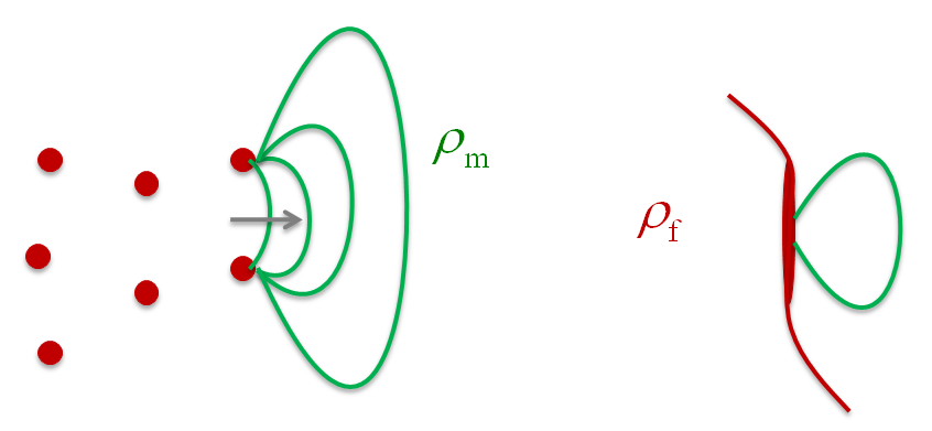
Figure 11.3:Generation of mobile dislocation, by forest dislocations.
Mobile dislocations can be immobilized by binary interactions (see Figure 11.4). The contributions to the evolution equations therefore have the following form: and , with the condition .
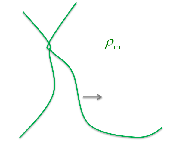
Figure 11.4:Immobilization of mobile dislocation by binary interactions.
Mobile dislocations can be immobilized through interaction with forest dislocations (see Figure 11.5). If the characteristic distance between forest dislocations is , then it takes a dislocation with velocity a certain amount of time to encounter such a forest dislocation, . The contributions to the evolution equations therefore have the following form: and , with the condition .
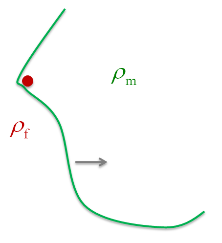
Figure 11.5:Immobilization of mobile dislocation through interaction with forest interactions.
Forest dislocations can be re-distributed or annihilated when plastic deformation occurs (see Figure 11.6). The contributions to the evolution equations therefore have the following form: and .
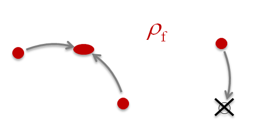
Figure 11.6:Re-distribution and annihilation of forest interactions.


If we combine all of these contributions to the evolution equations, we obtain the following non-linear system:
with constants . This is a set of evolution equations proposed by Estrin and Kubin (1986) and Estrin (1996). It needs to be completed by an expression for the magnitude of the dislocation velocity . This can either be done with detailed dislocation simulations, for given loading conditions. However, if one does not want to resolve to such detailed and involved simulations, one may also proceed as follows:
For a metal, the plastic strain rate is of the form
where (according to (11.7)), is also given by . While the critical stress is proportional to , it may be reasonable to assume that is proportional to . Therefore, one finds
with a constant .
In summary, the set of evolution equations (11.8), (11.9), and (11.11) allows to solve the evolution of dislocation densities and for a constant stress , in other words: in creep.
If on the other hand, one is interested in doing an experiment at constant applied strain rate , one can proceed as follows: Assuming linear elastic response, one has , and therefore the evolution of the stress is given by . Inserting the relation with velocity (11.11) one obtains
Therefore, for given constant , the set of evolution equations (11.8), (11.9) needs to be solved with velocity in (11.11) (as in the creep-case), but for constant strain-rate one needs to calculate the stress in (11.11) as a result of the dynamics (11.12). In short, one needs to solve three coupled differential equations for the variables , , and .
To close that chapter, we summarize that in the case of metal crystal plasticity, one can establish a rather detailed connection between the macroscopic modeling of viscoplasticity (in other words: ) and the structure evolution on the dislocation level.