

9 Structure quantification
The mechanical behavior of materials has its origin in the underlying microstructure. A lot of experimental efforts are currently undertaken to research and highlight the relation between the structure and the properties. In order to put such analysis on a solid basis, as well as to be able to capture the structure quantitatively in a model, methods for structure quantification must be employed. In this Chapter, we discuss some of the most important tools, namely:
Number density: Whenever defects or foreign particles are put in a material, their number density is an essential quantification tool.
Orientation distribution: If the defects are non-spherical, one might want to quantify the orientation distribution, e.g. the orientation of dislocation line-segments, or of fibers.
Transient space filling: If the filler particles do not change size, then the space filling (meaning: volume fraction) is constant. However, if the quantities of interest are growing crystals (for example in a semi-crystalline polymer, or in a solidifying metal), one may want to track and quantify the structure change.
9.1Number density
In 1D, the number density measures the number of particles per unit length. Therefore, the quantity tells how many particles are present in a segment of length located at position .
In 2D or 3D, the number density measures the number of particles per unit volume. Therefore, the quantity tells how many particles are present in a volume element of size (2D), or (3D), located at .
The quantity is closely related to the mass density . Particularly, if the objects of interest are identical particles of mass , we have
If furthermore we use that the (current) mass density is related to the mass density in the undeformed state through with of deformation gradient , one obtains
We have seen in Kinematics that the evolution of is given by the material time derivative . Using the chain-rule, we get for the number density
Formulated in terms of the spatial time derivative, one obtains
in complete analogy to the evolution equation for the mass density.
9.2Pair-correlation function
While the number density quantifies the number of particles per unit volume, it gives no information about how these particles are arranged with respect to each other (for example: crystalline, liquid-like, ...). In order to quantify the structure in this additional respect, the pair-correlation function is a common tool. The pair-correlation function is defined according to the following procedure:
Consider for each particle only its center-position. Situate yourself on one of the (point)-particles, . Then you measure how many other particles have a distance smaller than from you. You call this number of particles .
You now measure how many particles are at a distance between and away from you. This may be written as (see Figure 9.1).
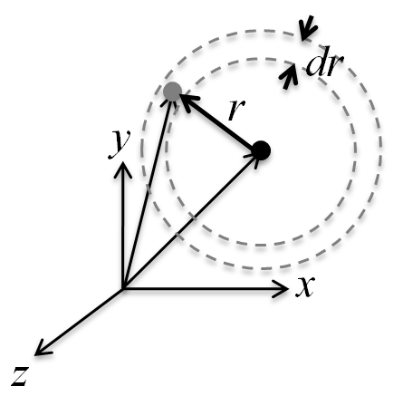
Figure 9.1:Illustration of the definition of the pair-correlation function.
You want to compare the measured for your real system with the same measurement on a system where the particles are distributed completely homogeneously at the density . You may thus write , and correspondingly .
The pair-correlation function of particle is then defined by the ratio of the actually measured to the homogeneous case, ,
You repeat this procedure for any other particle , and average over all of them (symbol ), to obtain the actual pair-correlation function of the system:
where the approximate signs apply if is much smaller than the characteristic length scale in the system.

As an example, the typical pair-correlation function for a fluid is shown in Figure 9.2. The fact that the particles have a finite size is clearly noticeable: vanishes for small , meaning that there are no particle pairs that have a so small center-center distance. At slightly larger distances, there is a first peak, which stands for the characteristic nearest-neighbor distance. For even larger values of , there are further but weaker peaks, representative of a weaker ordering on longer length scales.
It is left as an exercise to the reader to study the characteristic features in the pair-correlation function of (i) a homogeneous distribution of particle centers, (ii) a crystal in 1D, (iii) a simple cubic crystal in 3D, (iv) hard non-interacting particles of finite size in 1D, and (v) hard non-interacting particles of finite size in 2D.

Figure 9.2:Pair-correlation function for a typical fluid.
9.3Orientation-distribution function
For particles that are not purely spherical, it is also interesting to describe (beyond their number density and pair-correlation function) their orientation. This is done usually with the help of a so-called orientation-distribution function.
In order to describe the orientation of a rod (we consider a rod as a prototypical non-spherical particle in this entire section) in 2D, one needs only one degree of freedom, for example the angle with , see Figure 9.3. The orientation of the rod can then be described by
As a consequence, it is straightforward to show that the length of equals unity,

Figure 9.3:Definition of the orientation angle .
The orientation-distribution function for an fully isotropic system in 2D is given by , in other words, it is constant. The normalization constant can be determined from the condition that “The chance of finding the rod at any angle must be unity (=100%)”:
Question for the reader: How does the orientation-distribution look like for a fully oriented 2D system?
We mention that the situation in 3D is slightly more involved, since the description of an orientation vector requires two independent variables, and (see Figure 9.4), with and .

Figure 9.4:Definition of the orientation angles and .
The orientation of the rod can then be described by
As a consequence, it is straightforward to show that the length of equals unity,
The normalization condition for the 3D case is given by
One can show that for a fully isotropic structure in 3D, the orientation distribution function is given by . While the angle is homogeneously distributed ( does not depend on ), the angle has a low probability at the poles and the highest probability at the equator.
9.4Transient space filling
In many systems one deals with structures that are changing in time. Changes in time can occur because particles relocate and/or reorient in the sample. Another reason for structural changes is that the particles themselves change. For example, imagine a semi-crystalline polymer or a metal that is brought to a temperature below the crystallization temperature. In this case, crystals will form, and subsequently grow. As a result, the volume fraction of solid material changes over time. The description of such processes is the topic of this section.
Imagine particles in an observation volume , and let the particle volume be . If we disregard the possibility of overlapping/impinging particles, the volume fraction at a certain moment in time is given by
In the case where all particles are spheres of potentially different size , the volume fraction expression takes the form
Let us now consider the time evolution of the volume fraction. Using the chain rule, one obtains
which means that the volume fraction changes because the particles change their size.
It is reasonable to assume that the radial growth rate is actually the same for all particles, since the crystallization kinetics locally on the particle surface does not depend on the size of the entire particle. Therefore, we may write
where we have defined the surface per unit volume as
In the evolution equation (9.16) on notices that the volume (fraction) has a rate of change that is proportional to the area (per unit volume). This makes perfect sense since crystallization occurs by solidifying material at the already existing crystal surface.
For practical (numerical) application of (9.16), it is noteworthy that can not be expressed in terms of . Therefore, the evolution equation (9.16) is not a closed-form equation for . One needs the input of .
Finally, we comment on the fact that for constant crystallization conditions (in other words: constant ) the volume fraction grows beyond any limit. Particularly, it can become larger than unity, , which is clearly unphysical. The origin of this behavior is that we have not taken special care of the fact that the crystals may grow to a size where they begin to touch and even impinge on each other. In order to take this effect into account, it has been shown in the literature to be sufficient to correct for that by relating to the real volume fraction in terms of
In the limit of , we find (by using the Taylor-expansion). In the other limit of , one obtains , as required (see Figure 9.5). In order to compare with experimental measurements, must be used, rather than .

Figure 9.5:Strongly non-linear relation between the real volume fraction and the unbound volume fraction .