

4 Hyperelasticity
In this chapter the constitutive equations for elastic materials are discussed. Here only hyperelastic, and not hypoelastic material models are discussed. The hypoelastic models do not conserve energy and therefore are wrong from a thermodynamic perspective.
4.1Free energy
Hyperelastic materials[1] are materials for which the constitutive equation is defined in terms of a free energy function . This energy function depends on the deformation through the local deformation gradient only, i.e. .
The principle of objectivity requires that the stored energy is independent of rigid rotations which are applied to the current configuration. Hence it must hold that
This restriction implies that the stored-energy function can only depend on through the right Cauchy-Green deformation tensor
For elastic materials, described according to this energy potential, the following classical derivation holds
In the sequel of this chapter, attention will be focused on isotropic materials. For these materials, the stored-energy function may not depend on the orientation of the reference configuration, and hence only depends on the invariants of . For isotropic materials, it is therefore trivial to rephrase are the Cauchy stress tensor in terms of the left Cauchy-Green deformation tensor (the invariants are equal).
The energy density or stored-energy function cannot be chosen freely. The following restrictions apply
The stored-energy function must equal zero in the reference configuration.
The Cauchy stress tensor vanishes in the reference configuration.
For infinitesimal strains, the associated constitutive equation must equal the constitutive relation of an isotropic linear elastic material.
Infinitely large strains must lead to infinitely large values of . If one of the principal stretches tends to zero or infinity, the stored-energy function must tend to infinity. Hence, also if or it must hold that
4.2The incompressible Neo-Hookean model
The Neo-Hookean model provides a reasonable description of the behaviour of rubber like materials at finite strains.
The incompressible Neo-Hookean model is a particular case for which a kinematic constraint exist and for which the equations (4.3) may not be applied ad hoc.
It can be shown that the Cauchy stress tensor has a hydrostatic part that equals , where is a pressure variable. The second part of the Cauchy stress tensor is the extra stress part , for which (4.3) is applicable:
The extra stress tensor is generally not deviatoric. The stored-energy function for this material typically reads
The extra stress tensor is then linearly related to the Finger tensor. One may then write
where denotes the shear modulus. The strain measure has been chosen such that if no deformation is applied (e.g. ) the strain . Alternatively, the definition
is often used as well. This is justified because for incompressible materials the pressure is defined up to an arbitrary constant. The latter relation for the extra stress tensor can be easily derived from with the use of (4.3).
4.2.1Interpretation: simple shear
In case of simple shear the deformation tensor satisfies:
where is the applied shear. For this case the Finger tensor equals
Hence, the Cauchy stresses satisfy
One observes that the shear stress is linear with respect to the applied shear, regardless of its magnitude.
4.2.2Interpretation: uniaxial elongation
The uniaxial elongation of an incompressible solid is described by the following deformation tensor:
The Finger strain tensor satisfies
Consequently, the Cauchy stress tensor is given by, assuming ,
However, by definition in an uniaxial experiment, , hence
from which is follows that
Therefore the Cauchy stress in the principal stretch direction is given by
Figure 4.1 shows as a function of the stretch .
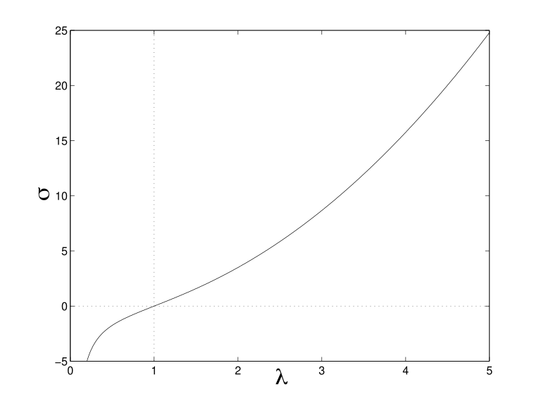
Figure 4.1:The non-dimensional Cauchy stress as a function of the stretch for the neo-Hookean model during uniaxial elongation
4.3Incompressible general elastic solid
The Neo-Hookean material model is only a first order approximation to the constitutive behaviour of elastic solids, and even for the description of the tensile test of rubbers is fails at moderate values of extension. A more general formulation would be of the form
Hence, the extra stress tensor is written as some function of the Finger tensor. This expression may be approximated by a power series:
with scalar constants. We may simplify this series with the help of the so-called Cayley-Hamilton theorem, which states that for any tensor it holds that
Higher powers of can also be expressed in terms of lower powers and invariants of . By multiplication of the Cayley Hamilton equations with one obtains:
Substitution of this into eq. (4.19) demonstrates that the third power of can be expressed in terms of and its inverse , giving
By using this, the series approximation can be rewritten as
where are scalar functions of the invariants of . For incompressible materials, the term may be accounted for by the pressure parameter , since this parameter is defined up to an arbitrary constant. Furthermore, in this case , hence a general expression of such a material is
The neo-Hookean solid is a special case of eq. (4.23): and .
4.4Compressible Neo-Hookean elastic solid
For compressible solids, the Kirchhoff stress tensor no longer equals the Cauchy stress tensor, and care must be taken with the use of equation (4.3) which now applies to .
4.4.1The deviatoric-volumetric multiplicative split
Infinitesimal theories use a standard additive split of the strain tensor into a volumetric part and a deviatoric part. For large deformations, this additive decomposition no longer corresponds to the physical interpretation which is commonly given to it, i.e. the deviatoric part is no longer volume preserving. By definition equals the volume ratio
The correct split now takes the following multiplicative form
A volume preserving, or isochoric, deformation tensor[2] is separated from the volumetric deformation . This means that
hence is incompressible. Therefore, the volumetric response can be associated with solely. Accordingly, isochoric deformation tensors may be defined, i.e. the isochoric Finger tensor
and the isochoric right Cauchy-Green deformation tensor
4.4.2Constitutive relations
A suitable generalization of the incompressible neo-Hookean material model to accommodate for compressibility is given by:
which corresponds to a stored-energy function that is given by
A large number of hyperelastic constitutive relations may thus be constructed. Another example is given by
with a stored-energy function
Another choice for is
Both choices (eq. (4.29) and eq. (4.31)) are admissible. The first choice for the extra stress tensor () yields a distortional stored-energy that is not isochoric, while the second () gives a that is isochoric. In what follows we shall therefore use the second choice.
Hyperelastic relations that involve can also be derived easily. An example of an extra stress tensor of this type is given by
4.5Relation to infinitesimal linear elasticity
In terms of displacements , the deformation tensor may be written as
Furthermore, the gradient operator with respect to the reference configuration is related to the gradient operator with respect to the current configuration via
For sufficiently small it can be seen by using eq. (4.35) that . Hence the deformation tensor may be approximated by
4.5.1Incompressible neo-Hookean solid.
Consequently the Finger strain tensor is approximated by
Hence in case of the incompressible neo-Hookean solid, the extra stress tensor is written as
Since the infinitesimal strain tensor is given by
this may also be written as
4.5.2Compressible neo-Hookean solid.
For sufficiently small , the volume ratio is approximated by
Therefore, the isochoric deformation tensor can be approximated by
Use is made of the Taylor series expansion . This implies that the isochoric Finger tensor follows from
Further,
Hence,
As a result the compressible neo-Hookean constitutive model may be approximated by
which is precisely the infinitesimal linear elastic constitutive model.