Vector and tensor calculus
In this chapter, attention is given to the definition and manipulation of vector and tensor fields. This mathematical description is used in many physical disciplines, and mechanics in particular. Vectors and tensors enable a compact notation and manipulation, without the necessity to resort to individual components with respect to a particular basis. The latter is needed only at the point that quantitative calculations need to be done, which is generally postponed to the last step. Special attention is given to Cartesian tensor calculus, which provides the basis for the elaboration of coordinate-free equations. Within this specific framework, no distinction is made between contravariant and covariant tensors while the metric tensor is not introduced neither. The quantification into components
measured with respect to a specific basis, and the related matrix calculus is also elaborated.
A.1 Scalars ¶ A scalar a a a T T T ρ \rho ρ
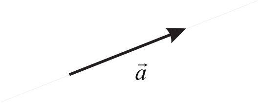
A.2 Vectors ¶ A.2.1 Definition ¶ A vector is a physical quantity possessing both a magnitude (or length)
and a direction.
Figure A.1: Magnitude and direction of a vector a ⃗ \V{a} a
In case of a vector a ⃗ \V{a} a
a ⃗ = ∥ a ⃗ ∥ e ⃗ \V{a} \;=\; \| \V{a} \| \V{e} a = ∥ a ∥ e the length is given by ∥ a ⃗ ∥ \|\V{a}\| ∥ a ∥ unit
vector e ⃗ \V{e} e zero vector 0 ⃗ \V{0} 0 a ⃗ \V{a} a
a ⃗ ⟹ a i \V{a} \;\Longrightarrow\; a_i a ⟹ a i A vector is thus indicated with a single index (i.c. i i i tensor (i.e. 1) thus equals its number of
indices. The index notation obtains a specific meaning once a basis has been chosen, since
the components of a vector are trivially identified with this notation,
see Section A.2.3
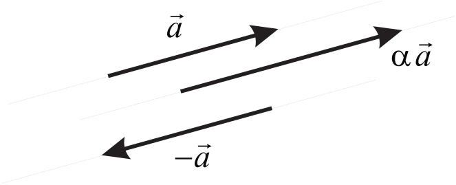
A.2.2 Vector operations ¶ Multiplication of a vector a ⃗ = ∥ a ⃗ ∥ e ⃗ \V{a} = \|\V{a}\| \V{e} a = ∥ a ∥ e α \alpha α b ⃗ \V{b} b α ∥ a ⃗ ∥ \alpha \|\V{a}\| α ∥ a ∥ e ⃗ \V{e} e
b ⃗ = α a ⃗ \V{b} \;=\; \alpha \V{a} b = α a Figure A.2: Multiplication of a vector: b ⃗ = α a ⃗ \V{b} = \alpha\V{a} b = α a
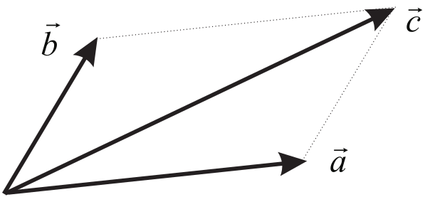
The sum of two vectors a ⃗ \V{a} a b ⃗ \V{b} b c ⃗ \V{c} c a ⃗ \V{a} a b ⃗ \V{b} b
c ⃗ = a ⃗ + b ⃗ \V{c} \;=\; \V{a} + \V{b} c = a + b Figure A.3: The sum of two vectors: c ⃗ = a ⃗ + b ⃗ \V{c}=\V{a}+\V{b} c = a + b
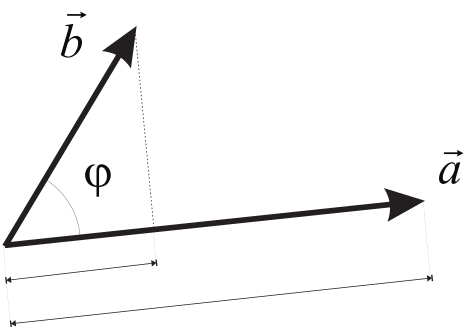
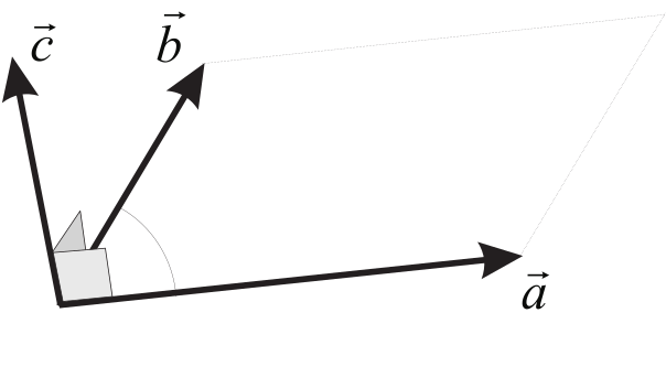
scalar product , inner product or dot product [1]
a ⃗ ⋅ b ⃗ = ∥ a ⃗ ∥ ∥ b ⃗ ∥ cos ( ϕ ) \V{a} \inp \V{b} \;=\; \| \V{a} \|\; \| \V{b} \| \cos(\phi) a ⋅ b = ∥ a ∥ ∥ b ∥ cos ( ϕ ) where ϕ \phi ϕ a ⃗ \V{a} a b ⃗ \V{b} b
Figure A.4: The inner product of two vectors: a ⃗ ⋅ b ⃗ \V{a}\inp\V{b} a ⋅ b
The product is commutative, i.e.:
a ⃗ ⋅ b ⃗ = b ⃗ ⋅ a ⃗ \V{a} \inp \V{b} \;=\; \V{b} \inp \V{a} a ⋅ b = b ⋅ a and linear
a ⃗ ⋅ ( b ⃗ + c ⃗ ) = a ⃗ ⋅ b ⃗ + a ⃗ ⋅ c ⃗ \V{a} \inp (\V{b} + \V{c}) \;=\; \V{a}\inp\V{b} + \V{a}\inp\V{c} a ⋅ ( b + c ) = a ⋅ b + a ⋅ c Using index notations, Einstein’s summation convention has to be
introduced. This convention states, that a summation is made over
all repeated indices, where the range of the summation equals the
dimension n n n
a ⃗ ⋅ b ⃗ = a i b i = ∑ i = 1 3 a i b i \V{a}\cdot\V{b} \;=\; a_ib_i \;=\; \sum_{i=1}^3 a_i b_i a ⋅ b = a i b i = i = 1 ∑ 3 a i b i The summation symbol is generally not written, but here simply added to clarify the
convention.
The scalar product of a vector with itself yields the square of its length:
a ⃗ ⋅ a ⃗ = ∥ a ⃗ ∥ 2 ≥ 0 \V{a} \inp \V{a} \;=\; \| \V{a} \|^2 \geq 0 a ⋅ a = ∥ a ∥ 2 ≥ 0 The vector product or cross product of two vectors is a
vector quantity:
a ⃗ × b ⃗ = c ⃗ \V{a} \cross \V{b} \;=\; \V{c} a × b = c The length of the vector c ⃗ \V{c} c
∥ c ⃗ ∥ = ∥ a ⃗ ∥ ∥ b ⃗ ∥ sin ( ϕ ) \| \V{c} \| \;=\; \| \V{a} \|\; \| \V{b} \| \sin(\phi) ∥ c ∥ = ∥ a ∥ ∥ b ∥ sin ( ϕ ) where ϕ \phi ϕ a ⃗ \V{a} a b ⃗ \V{b} b a ⃗ \V{a} a b ⃗ \V{b} b c ⃗ \V{c} c a ⃗ \V{a} a b ⃗ \V{b} b a ⃗ \V{a} a b ⃗ \V{b} b c ⃗ \V{c} c
Figure A.5: The cross product of two vectors: c ⃗ = a ⃗ × b ⃗ \V{c}=\V{a}\cross\V{b} c = a × b
The linearity of the vector product is expressed through
a ⃗ × ( b ⃗ + c ⃗ ) = a ⃗ × b ⃗ + a ⃗ × c ⃗ \V{a} \cross (\V{b} + \V{c}) \;=\; \V{a} \cross \V{b} + \V{a} \cross \V{c} a × ( b + c ) = a × b + a × c The vector product is not commutative:
b ⃗ × a ⃗ = − a ⃗ × b ⃗ \V{b} \cross \V{a} \;=\; - \V{a} \cross \V{b} b × a = − a × b which can be concluded from the definition. It can be shown that:
a ⃗ × ( b ⃗ × c ⃗ ) = ( a ⃗ ⋅ c ⃗ ) b ⃗ − ( a ⃗ ⋅ b ⃗ ) c ⃗ \V{a} \cross (\V{b} \cross \V{c}) \;=\;
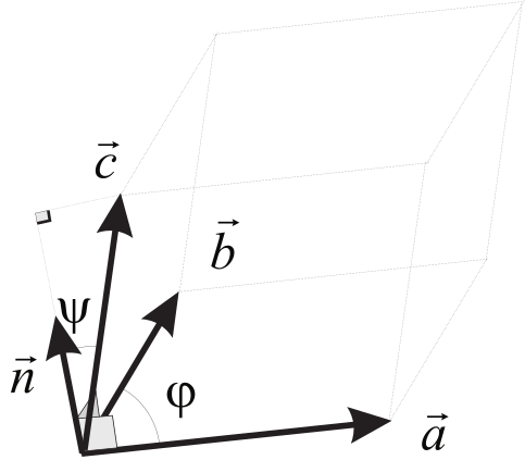
(\V{a} \inp \V{c}) \V{b} - (\V{a} \inp \V{b}) \V{c} a × ( b × c ) = ( a ⋅ c ) b − ( a ⋅ b ) c The triple product [2]
a ⃗ × b ⃗ ⋅ c ⃗ = ∥ a ⃗ ∥ ∥ b ⃗ ∥ sin ( ϕ ) ( n ⃗ ⋅ c ⃗ ) = ∥ a ⃗ ∥ ∥ b ⃗ ∥ sin ( ϕ ) ∥ c ⃗ ∥ cos ( ψ ) \begin{aligned}
\V{a} \cross \V{b} \inp \V{c} \;&\;=
\| \V{a} \|\; \| \V{b} \| \sin(\phi) (\V{n} \inp \V{c}) \\
\;&=\; \| \V{a} \|\; \| \V{b} \| \sin(\phi) \| \V{c} \| \cos(\psi)
\end{aligned} a × b ⋅ c = ∥ a ∥ ∥ b ∥ sin ( ϕ ) ( n ⋅ c ) = ∥ a ∥ ∥ b ∥ sin ( ϕ ) ∥ c ∥ cos ( ψ ) where n ⃗ \V{n} n a ⃗ × b ⃗ \V{a} \cross \V{b} a × b ϕ \phi ϕ a ⃗ \V{a} a b ⃗ \V{b} b ψ \psi ψ c ⃗ \V{c} c n ⃗ \V{n} n
Figure A.6: The triple product of three vectors a ⃗ × b ⃗ ⋅ c ⃗ \V{a}\cross\V{b}\inp\V{c} a × b ⋅ c
The absolute value of the triple product equals the volume of the parallelepiped spanned
by the three vectors. If a ⃗ × b ⃗ ⋅ c ⃗ ≠ 0 \V{a} \cross \V{b} \inp \V{c} \neq 0 a × b ⋅ c = 0 independent .
The tensor product [3] open
product of two vectors
a ⃗ b ⃗ \V{a}\V{b} a b dyad .
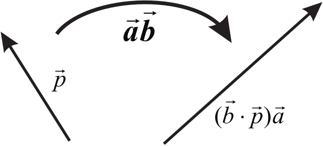
Application of the dyad a ⃗ b ⃗ \V{a}\V{b} a b p ⃗ \V{p} p a ⃗ \V{a} a ( b ⃗ ⋅ p ⃗ ) (\V{b} \inp \V{p}) ( b ⋅ p )
a ⃗ b ⃗ ⋅ p ⃗ = a ⃗ ( b ⃗ ⋅ p ⃗ ) \V{a}\V{b} \inp \V{p} \;=\; \V{a} (\V{b} \inp \V{p}) a b ⋅ p = a ( b ⋅ p ) or in index notation
( a i b j ) p j = a i ( b j p j ) (a_ib_j) p_j \;=\; a_i (b_jp_j) ( a i b j ) p j = a i ( b j p j ) Figure A.7: The tensor product: a ⃗ b ⃗ ⋅ p ⃗ \V{a} \V{b} \inp \V{p} a b ⋅ p
The linearity of the transformation is expressed by:
a ⃗ b ⃗ ⋅ ( α p ⃗ + β q ⃗ ) = α a ⃗ ( b ⃗ ⋅ p ⃗ ) + β a ⃗ ( b ⃗ ⋅ q ⃗ ) \V{a}\V{b} \inp ( \alpha \V{p} + \beta \V{q} ) \;=\;
\alpha \V{a} (\V{b} \inp \V{p}) + \beta \V{a} (\V{b} \inp \V{q}) a b ⋅ ( α p + β q ) = α a ( b ⋅ p ) + β a ( b ⋅ q ) The transpose of a dyad (also called conjugate dyad or adjoint
dyad )[4]
( a ⃗ b ⃗ ) T = b ⃗ a ⃗ ≠ a ⃗ b ⃗ ( \V{a}\V{b} )^T \;=\; \V{b}\V{a} \neq \V{a}\V{b} ( a b ) T = b a = a b If ( a ⃗ b ⃗ ) T = a ⃗ b ⃗ ( \V{a}\V{b} )^T = \V{a}\V{b} ( a b ) T = a b a ⃗ b ⃗ \V{a}\V{b} a b
A.2.3 Vector basis ¶ In three-dimensional space, a set of three vectors c ⃗ 1 \V{c}_1 c 1 c ⃗ 2 \V{c}_2 c 2 c ⃗ 3 \V{c}_3 c 3 basis , denoted by { c ⃗ 1 , c ⃗ 2 , c ⃗ 3 } \{ \V{c}_1, \V{c}_2, \V{c}_3 \} { c 1 , c 2 , c 3 }
{ c ⃗ 1 , c ⃗ 2 , c ⃗ 3 } ⇒ c ⃗ 1 × c ⃗ 2 ⋅ c ⃗ 3 ≠ 0 \{ \V{c}_1, \V{c}_2, \V{c}_3 \} \quad \Rightarrow \quad
\V{c}_1 \cross \V{c}_2 \inp \V{c}_3 \neq 0 { c 1 , c 2 , c 3 } ⇒ c 1 × c 2 ⋅ c 3 = 0 The three vectors c ⃗ 1 \V{c}_1 c 1 c ⃗ 2 \V{c}_2 c 2 c ⃗ 3 \V{c}_3 c 3 base vectors .
If the basis consists of mutually perpendicular vectors, the basis is
called an orthogonal basis .
If the basis consists of mutually perpendicular unit vectors, the basis is called an
orthonormal basis . In the latter case the base vectors are
usually denoted by e ⃗ 1 \V{e}_1 e 1 e ⃗ 2 \V{e}_2 e 2 e ⃗ 3 \V{e}_3 e 3
{ e ⃗ 1 , e ⃗ 2 , e ⃗ 3 } ⇒ e ⃗ i ⋅ e ⃗ j = δ i j = { 0 if i ≠ j 1 if i = j \basis \quad \Rightarrow \quad \V{e}_i \inp \V{e}_j \;=\; \delta_{ij}
\;=\; \left\{ \begin{array}{lcl}
0 & \mbox{if} & \mbox{$i \neq j$} \\
1 & \mbox{if} & \mbox{$i = j$}
\end{array}
\right. { e 1 , e 2 , e 3 } ⇒ e i ⋅ e j = δ ij = { 0 1 if if i = j i = j where δ i j \delta_{ij} δ ij Kronecker delta . A basis { e ⃗ 1 , e ⃗ 2 , e ⃗ 3 } \basis { e 1 , e 2 , e 3 } righthanded [5] e ⃗ 1 \V{e}_1 e 1 e ⃗ 2 \V{e}_2 e 2 e ⃗ 3 \V{e}_3 e 3
e ⃗ 1 × e ⃗ 2 = e ⃗ 3 e ⃗ 2 × e ⃗ 3 = e ⃗ 1 e ⃗ 3 × e ⃗ 1 = e ⃗ 2 \begin{aligned}
\V{e}_1 \cross \V{e}_2 \;&=\; \V{e}_3 \\
\V{e}_2 \cross \V{e}_3 \;&=\; \V{e}_1 \\
\V{e}_3 \cross \V{e}_1 \;&=\; \V{e}_2
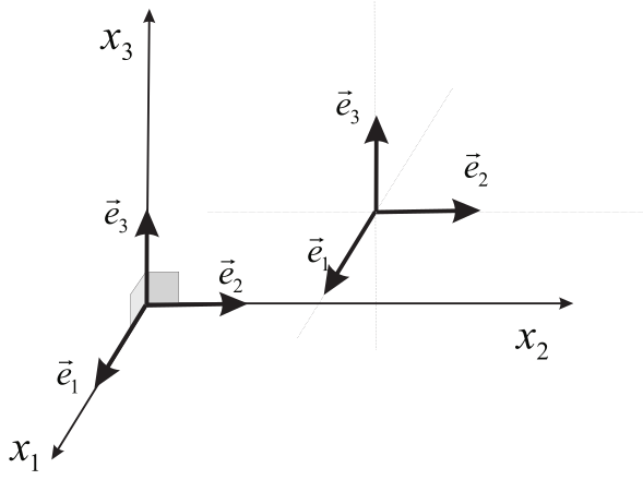
\end{aligned} e 1 × e 2 e 2 × e 3 e 3 × e 1 = e 3 = e 1 = e 2 A Cartesian basis is an orthonormal basis in which the base vectors
are independent of the location in three-dimensional space. It is
usually denoted by { e ⃗ 1 , e ⃗ 2 , e ⃗ 3 } \basis { e 1 , e 2 , e 3 } { e ⃗ x , e ⃗ y , e ⃗ z } \xyzbasis { e x , e y , e z }
Figure A.8: A Cartesian orthonormal basis { e ⃗ 1 , e ⃗ 2 , e ⃗ 3 } \basis { e 1 , e 2 , e 3 }
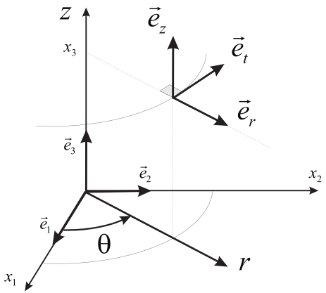
A cylindrical basis is an orthonormal basis as well. It is usually
denoted by { e ⃗ r , e ⃗ t , e ⃗ z } \cylbasis { e r , e t , e z } { e ⃗ 1 , e ⃗ 2 , e ⃗ 3 } \basis { e 1 , e 2 , e 3 } { e ⃗ r , e ⃗ t , e ⃗ z } \cylbasis { e r , e t , e z }
e ⃗ r ( θ ) = cos ( θ ) e ⃗ 1 + sin ( θ ) e ⃗ 2 e ⃗ t ( θ ) = − sin ( θ ) e ⃗ 1 + c o s ( θ ) e ⃗ 2 e ⃗ z = e ⃗ 3 \begin{aligned}
\V{e}_r(\theta) \;&=\; \cos(\theta) \V{e}_1 + \sin(\theta) \V{e}_2 \\
\V{e}_t(\theta) \;&=\; - \sin(\theta) \V{e}_1 + cos(\theta) \V{e}_2 \\
\V{e}_z \;&=\; \V{e}_3
\end{aligned} e r ( θ ) e t ( θ ) e z = cos ( θ ) e 1 + sin ( θ ) e 2 = − sin ( θ ) e 1 + cos ( θ ) e 2 = e 3 Figure A.9: A cylindrical orthonormal basis { e ⃗ r , e ⃗ t , e ⃗ z } \cylbasis { e r , e t , e z }
It is important to note that the base vectors
e ⃗ r \V{e}_r e r e ⃗ t \V{e}_t e t θ \theta θ θ \theta θ
d e ⃗ r ( θ ) d θ = e ⃗ t ( θ ) d e ⃗ t ( θ ) d θ = − e ⃗ r ( θ ) \begin{aligned}
\frac{d\V{e}_r(\theta)}{d\theta} \;&=\; \V{e}_t(\theta)\\
\frac{d\V{e}_t(\theta)}{d\theta} \;&=\; - \V{e}_r(\theta)
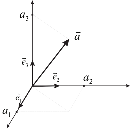
\end{aligned} d θ d e r ( θ ) d θ d e t ( θ ) = e t ( θ ) = − e r ( θ ) A.2.4 Vector components; matrix notation of a vector ¶ Let { c ⃗ 1 , c ⃗ 2 , c ⃗ 3 } \{ \V{c}_1, \V{c}_2, \V{c}_3 \} { c 1 , c 2 , c 3 } a ⃗ \V{a} a { e ⃗ 1 , e ⃗ 2 , e ⃗ 3 } \basis { e 1 , e 2 , e 3 }
a ⃗ = a 1 e ⃗ 1 + a 2 e ⃗ 2 + a 3 e ⃗ 3 = a i e ⃗ i , \V{a} \;=\; a_1 \V{e}_1 + a_2 \V{e}_2 + a_3 \V{e}_3 = a_i\V{e}_i, a = a 1 e 1 + a 2 e 2 + a 3 e 3 = a i e i , where we again used the Einstein summation convention , i.e. we sum over
the repeated index i i i
Figure A.10: Components a i a_i a i a ⃗ \V{a} a { e ⃗ 1 , e ⃗ 2 , e ⃗ 3 } \basis { e 1 , e 2 , e 3 }
The coefficients a i a_i a i components of the vector a ⃗ \V{a} a a i a_i a i a ⃗ \V{a} a e ⃗ i \V{e}_i e i
a i = a ⃗ ⋅ e ⃗ i a_i \;=\; \V{a}\inp\V{e}_i a i = a ⋅ e i The component a i a_i a i projection of the
vector a ⃗ \V{a} a e ⃗ i \V{e}_i e i matrix notation in which we
store base vectors and components in a column :
a ∼ = [ a 1 a 2 a 3 ] e ⃗ ∼ = [ e ⃗ 1 e ⃗ 2 e ⃗ 3 ] \begin{aligned}
\C{a} \;&=\; \begin{bmatrix} a_1 \\ a_2 \\ a_3 \end{bmatrix} \\
\C{\V{e}} \;&=\; \begin{bmatrix} \V{e}_1 \\ \V{e}_2 \\ \V{e}_3 \end{bmatrix}
\end{aligned} ∼ a ∼ e = ⎣ ⎡ a 1 a 2 a 3 ⎦ ⎤ = ⎣ ⎡ e 1 e 2 e 3 ⎦ ⎤ Thus we may write:
a ⃗ = [ a 1 a 2 a 3 ] [ e ⃗ 1 e ⃗ 2 e ⃗ 3 ] = a ∼ T e ⃗ ∼ \V{a} \;=\; \begin{bmatrix} a_1 & a_2 & a_3 \end{bmatrix}
\begin{bmatrix} \V{e}_1 \\ \V{e}_2 \\ \V{e}_3 \end{bmatrix} \;=\;
\C{a}^T \C{\V{e}} a = [ a 1 a 2 a 3 ] ⎣ ⎡ e 1 e 2 e 3 ⎦ ⎤ = ∼ a T ∼ e or, equivalently:
a ⃗ = [ e ⃗ 1 e ⃗ 2 e ⃗ 3 ] [ a 1 a 2 a 3 ] = e ⃗ ∼ T a ∼ \V{a} \;=\; \begin{bmatrix} \V{e}_1 & \V{e}_2 & \V{e}_3 \end{bmatrix}
\begin{bmatrix} a_1 \\ a_2 \\ a_3 \end{bmatrix} =
\C{\V{e}}^T \C{a} a = [ e 1 e 2 e 3 ] ⎣ ⎡ a 1 a 2 a 3 ⎦ ⎤ = ∼ e T ∼ a The relations a i = a ⃗ ⋅ e ⃗ i a_i = \V{a}\inp\V{e}_i a i = a ⋅ e i
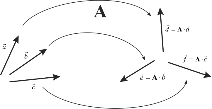
a ∼ = a ⃗ ⋅ e ⃗ ∼ \C{a} \;=\; \V{a}\inp\C{\V{e}} ∼ a = a ⋅ ∼ e A.3 Second order tensors ¶ A.3.1 Definition ¶ A second order tensor is a linear transformation of a vector
into another vector:
A ⋅ p ⃗ = q ⃗ \T{A} \inp \V{p} \;=\; \V{q} A ⋅ p = q or in index notation
A i j p j = q i A_{ij}p_j \;=\; q_i A ij p j = q i Note that we limit ourselves here to so-called Cartesian tensors, which allow orthogonal
linear coordinate transformations only. In a three-dimensional space, a second-order
tensor is fully defined by the image of three independent vectors, see
Figure A.11
Figure A.11: A second-order tensor A \T{A} A
Indeed, any set of three independent vectors constitutes a vector basis by means of which
any other vector can be expressed. The image of an arbitrary vector can be found
trivially through the images of three such vectors. This property is a direct consequence
of the linearity of the transformation, which is expressed by:
A ⋅ ( α m ⃗ + β n ⃗ ) = α A ⋅ m ⃗ + β A ⋅ n ⃗ \T{A} \inp ( \alpha \V{m} + \beta \V{n} ) \;=\;
\alpha \T{A} \inp \V{m} + \beta \T{A} \inp \V{n} A ⋅ ( α m + β n ) = α A ⋅ m + β A ⋅ n For an arbitrary vector a ⃗ = a 1 e ⃗ 1 + a 2 e ⃗ 2 + a 3 e ⃗ 3 \V{a}=a_1\V{e}_1 + a_2\V{e}_2 + a_3\V{e}_3 a = a 1 e 1 + a 2 e 2 + a 3 e 3
A ⋅ a ⃗ = a 1 ( A ⋅ e ⃗ 1 ) + a 2 ( A ⋅ e ⃗ 2 ) + a 3 ( A ⋅ e ⃗ 3 ) \T{A}\inp\V{a} \;=\; a_1(\T{A}\inp\V{e}_1) + a_2(\T{A}\inp\V{e}_2) + a_3(\T{A}\inp\V{e}_3) A ⋅ a = a 1 ( A ⋅ e 1 ) + a 2 ( A ⋅ e 2 ) + a 3 ( A ⋅ e 3 ) A.3.2 Some properties ¶ Any second order tensor may be represented by a finite, nonunique, sum of dyads:
A = α 1 a ⃗ 1 b ⃗ 1 + α 2 a ⃗ 2 b ⃗ 2 + α 3 a ⃗ 3 b ⃗ 3 + … \T{A} \;=\;
\alpha_1 \V{a}_1 \V{b}_1 + \alpha_2 \V{a}_2 \V{b}_2 +
\alpha_3 \V{a}_3 \V{b}_3 + \dots A = α 1 a 1 b 1 + α 2 a 2 b 2 + α 3 a 3 b 3 + … Two special tensors are the zero tensor O \T{O} O unit tensor [6] I \T{I} I p ⃗ \V{p} p
O ⋅ p ⃗ = 0 ⃗ \T{O} \inp \V{p} \;=\; \V{0} O ⋅ p = 0 I ⋅ p ⃗ = p ⃗ \T{I} \inp \V{p} \;=\; \V{p} I ⋅ p = p The index notations for O \T{O} O I \T{I} I
0 ⇔ 0 i j I ⇔ δ i j \begin{aligned}
\T{0} \;&\Leftrightarrow\; 0_{ij}\\
\T{I} \;&\Leftrightarrow\; \delta_{ij}
\end{aligned} 0 I ⇔ 0 ij ⇔ δ ij where the Kronecker delta δ i j \delta_{ij} δ ij
The transpose or conjugate A T \T{A}^T A T A \T{A} A
A T ⋅ p ⃗ = p ⃗ ⋅ A \T{A}^T \inp \V{p} \;=\; \V{p} \inp \T{A} A T ⋅ p = p ⋅ A In index notation it holds that
A ⇔ A i j ⟹ A T ⇔ A j i \T{A}\;\Leftrightarrow\;A_{ij} \quad\Longrightarrow\quad \T{A}^T\;\Leftrightarrow\;A_{ji} A ⇔ A ij ⟹ A T ⇔ A ji For the special case A = a ⃗ b ⃗ \T{A} = \V{a}\V{b} A = a b
( a ⃗ b ⃗ ) T ⋅ p ⃗ = p ⃗ ⋅ ( a ⃗ b ⃗ ) = ( p ⃗ ⋅ a ⃗ ) b ⃗ = b ⃗ ( p ⃗ ⋅ a ⃗ ) = b ⃗ ( a ⃗ ⋅ p ⃗ ) = ( b ⃗ a ⃗ ) ⋅ p ⃗ \begin{aligned}
(\V{a}\V{b})^T \inp \V{p} \;&=\; \V{p} \inp (\V{a}\V{b}) \\
\;&=\; (\V{p} \inp \V{a}) \V{b} \\
\;&=\; \V{b} (\V{p} \inp \V{a}) \\
\;&=\; \V{b} (\V{a} \inp \V{p}) \\
\;&=\; (\V{b} \V{a}) \inp \V{p}
\end{aligned} ( a b ) T ⋅ p = p ⋅ ( a b ) = ( p ⋅ a ) b = b ( p ⋅ a ) = b ( a ⋅ p ) = ( b a ) ⋅ p showing that:
( a ⃗ b ⃗ ) T = b ⃗ a ⃗ (\V{a}\V{b})^T \;=\; \V{b} \V{a} ( a b ) T = b a If A \T{A} A A T \T{A}^T A T
( α A ) ⋅ v ⃗ = A ⋅ ( α v ⃗ ) , ( A + B ) ⋅ v ⃗ = A ⋅ v ⃗ + B ⋅ v ⃗ , ( A ⋅ B ) ⋅ v ⃗ = A ⋅ ( B ⋅ v ⃗ ) \begin{aligned}
(\alpha \T{A}) \inp \V{v} \;&=\; \T{A} \inp (\alpha \V{v}) ,\\
(\T{A} + \T{B}) \inp \V{v} \;&=\; \T{A} \inp \V{v} + \T{B} \inp \V{v} ,\\
(\T{A}\inp\T{B})\inp\V{v} \;&=\; \T{A}\inp(\T{B}\inp\V{v})
\end{aligned} ( α A ) ⋅ v ( A + B ) ⋅ v ( A ⋅ B ) ⋅ v = A ⋅ ( α v ) , = A ⋅ v + B ⋅ v , = A ⋅ ( B ⋅ v ) Note that (in general):
A ⋅ B ≠ B ⋅ A \T{A}\inp\T{B} \;\neq\; \T{B}\inp\T{A} A ⋅ B = B ⋅ A The inner product of a tensor with itself is called the square of a tensor, i.e.
A 2 = A ⋅ A \T{A}^2 \;=\; \T{A}\inp\T{A} A 2 = A ⋅ A Likewise, higher-order exponents are defined through repeated inner products, e.g.,
A 3 = A ⋅ A ⋅ A \T{A}^3 \;=\; \T{A}\inp\T{A}\inp\T{A} A 3 = A ⋅ A ⋅ A A.3.3 Tensor components; matrix notation of a tensor ¶ Consider a three-dimensional space with a basis { e ⃗ 1 , e ⃗ 2 , e ⃗ 3 } \basis { e 1 , e 2 , e 3 } (A.25) a ⃗ i \V{a}_i a i b ⃗ i \V{b}_i b i (A.35) (A.35)
A = A 11 e ⃗ 1 e ⃗ 1 + A 12 e ⃗ 1 e ⃗ 2 + A 13 e ⃗ 1 e ⃗ 3 + A 21 e ⃗ 2 e ⃗ 1 + A 22 e ⃗ 2 e ⃗ 2 + A 23 e ⃗ 2 e ⃗ 3 + A 31 e ⃗ 3 e ⃗ 1 + A 32 e ⃗ 3 e ⃗ 2 + A 33 e ⃗ 3 e ⃗ 3 \begin{aligned}
\T{A} \;=\; & A_{11}\V{e}_1\V{e}_1 + A_{12}\V{e}_1\V{e}_2 + A_{13}\V{e}_1\V{e}_3 + \\
& A_{21}\V{e}_2\V{e}_1 + A_{22}\V{e}_2\V{e}_2 + A_{23}\V{e}_2\V{e}_3 + \\
& A_{31}\V{e}_3\V{e}_1 + A_{32}\V{e}_3\V{e}_2 + A_{33}\V{e}_3\V{e}_3
\end{aligned} A = A 11 e 1 e 1 + A 12 e 1 e 2 + A 13 e 1 e 3 + A 21 e 2 e 1 + A 22 e 2 e 2 + A 23 e 2 e 3 + A 31 e 3 e 1 + A 32 e 3 e 2 + A 33 e 3 e 3 where the coefficients A i j A_{ij} A ij α i \alpha_i α i a ⃗ \V{a} a b ⃗ \V{b} b A \T{A} A A i j A_{ij} A ij components of the tensor A \T{A} A { e ⃗ 1 , e ⃗ 2 , e ⃗ 3 } \basis { e 1 , e 2 , e 3 } A i j A_{ij} A ij A \T{A} A
A i j = e ⃗ i ⋅ A ⋅ e ⃗ j A_{ij} \;=\; \V{e}_i \inp \T{A} \inp \V{e}_j A ij = e i ⋅ A ⋅ e j as can be verified from substitution of (A.47) A i j A_{ij} A ij matrix A ‾ \M{A} A
A ‾ = [ A 11 A 12 A 13 A 21 A 22 A 23 A 31 A 32 A 33 ] = [ ( e ⃗ 1 ⋅ A ⋅ e ⃗ 1 ) ( e ⃗ 1 ⋅ A ⋅ e ⃗ 2 ) ( e ⃗ 1 ⋅ A ⋅ e ⃗ 3 ) ( e ⃗ 2 ⋅ A ⋅ e ⃗ 1 ) ( e ⃗ 2 ⋅ A ⋅ e ⃗ 2 ) ( e ⃗ 2 ⋅ A ⋅ e ⃗ 3 ) ( e ⃗ 3 ⋅ A ⋅ e ⃗ 1 ) ( e ⃗ 3 ⋅ A ⋅ e ⃗ 2 ) ( e ⃗ 3 ⋅ A ⋅ e ⃗ 3 ) ] = [ e ⃗ 1 e ⃗ 2 e ⃗ 3 ] ⋅ A ⋅ [ e ⃗ 1 e ⃗ 2 e ⃗ 3 ] = e ⃗ ∼ ⋅ A ⋅ e ⃗ ∼ T \begin{aligned}
\M{A}
\;&=\;
\begin{bmatrix}
A_{11} & A_{12} & A_{13} \\
A_{21} & A_{22} & A_{23} \\
A_{31} & A_{32} & A_{33}
\end{bmatrix} \\
\;&=\; \begin{bmatrix}
(\V{e}_1 \inp \T{A} \inp \V{e}_1) & (\V{e}_1 \inp \T{A} \inp \V{e}_2) &
(\V{e}_1 \inp \T{A} \inp \V{e}_3) \\
(\V{e}_2 \inp \T{A} \inp \V{e}_1) & (\V{e}_2 \inp \T{A} \inp \V{e}_2) &
(\V{e}_2 \inp \T{A} \inp \V{e}_3) \\
(\V{e}_3 \inp \T{A} \inp \V{e}_1) & (\V{e}_3 \inp \T{A} \inp \V{e}_2) &
(\V{e}_3 \inp \T{A} \inp \V{e}_3)
\end{bmatrix} \\
\;&=\; \begin{bmatrix} \V{e}_1 \\ \V{e}_2 \\ \V{e}_3 \end{bmatrix} \inp
\T{A} \inp \begin{bmatrix} \V{e}_1 & \V{e}_2 & \V{e}_3 \end{bmatrix} \\
\;&=\; \C{\V{e}} \inp \T{A} \inp \C{\V{e}}^T
\end{aligned} A = ⎣ ⎡ A 11 A 21 A 31 A 12 A 22 A 32 A 13 A 23 A 33 ⎦ ⎤ = ⎣ ⎡ ( e 1 ⋅ A ⋅ e 1 ) ( e 2 ⋅ A ⋅ e 1 ) ( e 3 ⋅ A ⋅ e 1 ) ( e 1 ⋅ A ⋅ e 2 ) ( e 2 ⋅ A ⋅ e 2 ) ( e 3 ⋅ A ⋅ e 2 ) ( e 1 ⋅ A ⋅ e 3 ) ( e 2 ⋅ A ⋅ e 3 ) ( e 3 ⋅ A ⋅ e 3 ) ⎦ ⎤ = ⎣ ⎡ e 1 e 2 e 3 ⎦ ⎤ ⋅ A ⋅ [ e 1 e 2 e 3 ] = ∼ e ⋅ A ⋅ ∼ e T Using the matrix A ‾ \M{A} A (A.47)
A = [ e ⃗ 1 e ⃗ 2 e ⃗ 3 ] [ A 11 A 12 A 13 A 21 A 22 A 23 A 31 A 32 A 33 ] [ e ⃗ 1 e ⃗ 2 e ⃗ 3 ] = e ⃗ ∼ T A ‾ e ⃗ ∼ \begin{aligned}
\T{A} \;&=\; \begin{bmatrix} \V{e}_1 & \V{e}_2 & \V{e}_3 \end{bmatrix}
\begin{bmatrix} A_{11} & A_{12} & A_{13} \\
A_{21} & A_{22} & A_{23} \\
A_{31} & A_{32} & A_{33} \end{bmatrix}
\begin{bmatrix} \V{e}_1 \\ \V{e}_2 \\ \V{e}_3 \end{bmatrix} \\
\;&=\; \C{\V{e}}^T \M{A} \; \C{\V{e}}
\end{aligned} A = [ e 1 e 2 e 3 ] ⎣ ⎡ A 11 A 21 A 31 A 12 A 22 A 32 A 13 A 23 A 33 ⎦ ⎤ ⎣ ⎡ e 1 e 2 e 3 ⎦ ⎤ = ∼ e T A ∼ e Together, equations (A.49) (A.50)
In (A.37) unit tensor I \T{I} I I \T{I} I (A.47) (A.37)
I = e ⃗ 1 e ⃗ 1 + e ⃗ 2 e ⃗ 2 + e ⃗ 3 e ⃗ 3 \T{I} \;=\; \V{e}_1\V{e}_1 + \V{e}_2\V{e}_2 + \V{e}_3\V{e}_3 I = e 1 e 1 + e 2 e 2 + e 3 e 3 Thus, for the unit matrix I ‾ \M{I} I unit tensor I \T{I} I
I ‾ = e ⃗ ∼ ⋅ e ⃗ ∼ T = [ 1 0 0 0 1 0 0 0 1 ] \M{I} \;=\; \C{\V{e}}\inp\C{\V{e}}^T =
\begin{bmatrix} 1 & 0 & 0 \\ 0 & 1 & 0 \\ 0 & 0 & 1 \end{bmatrix} I = ∼ e ⋅ ∼ e T = ⎣ ⎡ 1 0 0 0 1 0 0 0 1 ⎦ ⎤ A.3.4 Scalar functions of a tensor ¶ A.3.4.1 Euclidean norm ¶ The Euclidean norm [7] m m m
m = ∥ A ∥ = max e ⃗ ∥ A ⋅ e ⃗ ∥ ∀ e ⃗ with ∥ e ⃗ ∥ = 1. m \;=\; \| \T{A} \| = \max_{\V{e}} \| \T{A} \inp \V{e} \| \quad \forall\;
\V{e} \text{ with } \| \V{e} \| = 1 . m = ∥ A ∥ = e max ∥ A ⋅ e ∥ ∀ e with ∥ e ∥ = 1. The norm is an invariant quantity [8]
∥ A ∥ ≥ 0 ∥ α A ∥ = ∣ α ∣ ∥ A ∥ ∥ A ⋅ B ∥ ≤ ∥ A ∥ ∥ B ∥ ∥ A + B ∥ ≤ ∥ A ∥ + ∥ B ∥ \begin{aligned}
\| \T{A} \| \;&\geq\; 0 \\
\| \alpha \T{A} \| \;&=\; |\alpha|\; \| \T{A} \| \\
\| \T{A} \inp \T{B} \| \;&\leq\; \| \T{A} \|\; \| \T{B} \| \\
\| \T{A} + \T{B} \| \;&\leq\; \| \T{A} \| + \| \T{B} \|
\end{aligned} ∥ A ∥ ∥ α A ∥ ∥ A ⋅ B ∥ ∥ A + B ∥ ≥ 0 = ∣ α ∣ ∥ A ∥ ≤ ∥ A ∥ ∥ B ∥ ≤ ∥ A ∥ + ∥ B ∥ A.3.4.2 The first invariant ¶ The first invariant of a tensor A \T{A} A trace [9] A \T{A} A
J 1 ( A ) = tr ( A ) = 1 c ⃗ 1 × c ⃗ 2 ⋅ c ⃗ 3 [ c ⃗ 1 ⋅ A ⋅ ( c ⃗ 2 × c ⃗ 3 ) + c ⃗ 2 ⋅ A ⋅ ( c ⃗ 3 × c ⃗ 1 ) + c ⃗ 3 ⋅ A ⋅ ( c ⃗ 1 × c ⃗ 2 ) ] \begin{alignedat}{2}
J_1(\T{A}) \;&=\; \tr(\T{A}) && \\
&\;=\; \tfrac{1}{\V{c}_1 \cross \V{c}_2 \inp \V{c}_3}
[&& \V{c}_1 \inp \T{A} \inp ( \V{c}_2 \cross \V{c}_3 ) + \\
& && \V{c}_2 \inp \T{A} \inp ( \V{c}_3 \cross \V{c}_1 ) +
\V{c}_3 \inp \T{A} \inp ( \V{c}_1 \cross \V{c}_2 ) ]
\end{alignedat} J 1 ( A ) = tr ( A ) = c 1 × c 2 ⋅ c 3 1 [ c 1 ⋅ A ⋅ ( c 2 × c 3 ) + c 2 ⋅ A ⋅ ( c 3 × c 1 ) + c 3 ⋅ A ⋅ ( c 1 × c 2 )] where { c ⃗ 1 , c ⃗ 2 , c ⃗ 3 } \{ \V{c}_1, \V{c}_2, \V{c}_3 \} { c 1 , c 2 , c 3 } J 1 ( A ) J_1(\T{A}) J 1 ( A ) { e ⃗ 1 , e ⃗ 2 , e ⃗ 3 } \basis { e 1 , e 2 , e 3 }
J 1 ( A ) = e ⃗ 1 ⋅ A ⋅ e ⃗ 1 + e ⃗ 2 ⋅ A ⋅ e ⃗ 2 + e ⃗ 3 ⋅ A ⋅ e ⃗ 3 = A 11 + A 22 + A 33 = tr A ‾ \begin{aligned}
J_1(\T{A}) \;&=\;
\V{e}_1 \inp \T{A} \inp \V{e}_1 +
\V{e}_2 \inp \T{A} \inp \V{e}_2 +
\V{e}_3 \inp \T{A} \inp \V{e}_3 \\
\;&=\; A_{11} + A_{22} + A_{33}\\
\;&=\; \tr{\M{A}}
\end{aligned} J 1 ( A ) = e 1 ⋅ A ⋅ e 1 + e 2 ⋅ A ⋅ e 2 + e 3 ⋅ A ⋅ e 3 = A 11 + A 22 + A 33 = tr A The following properties hold for the first invariant:
J 1 ( A ) = J 1 ( A T ) J 1 ( I ) = 3 J 1 ( α A ) = α J 1 ( A ) J 1 ( A + B ) = J 1 ( A ) + J 1 ( B ) \begin{aligned}
J_1(\T{A}) \;&=\; J_1(\T{A}^T) \\
J_1(\T{I}) \;&=\; 3 \\
J_1(\alpha \T{A}) \;&=\; \alpha J_1(\T{A}) \\
J_1(\T{A} + \T{B}) \;&=\; J_1(\T{A}) + J_1(\T{B})
\end{aligned} J 1 ( A ) J 1 ( I ) J 1 ( α A ) J 1 ( A + B ) = J 1 ( A T ) = 3 = α J 1 ( A ) = J 1 ( A ) + J 1 ( B ) A.3.4.3 The second invariant ¶ The second invariant of a tensor A \T{A} A
J 2 ( A ) = 1 2 { tr 2 ( A ) − tr ( A 2 ) } = 1 c ⃗ 1 × c ⃗ 2 ⋅ c ⃗ 3 [ c ⃗ 1 ⋅ ( A ⋅ c ⃗ 2 ) × ( A ⋅ c ⃗ 3 ) + c ⃗ 2 ⋅ ( A ⋅ c ⃗ 3 ) × ( A ⋅ c ⃗ 1 ) + c ⃗ 3 ⋅ ( A ⋅ c ⃗ 1 ) × ( A ⋅ c ⃗ 2 ) ] \begin{alignedat}{2}
J_2(\T{A}) \;&=\; \half \{ \tr^2(\T{A}) - &&\tr(\T{A}^2) \} \\
\;&=\; \tfrac{1}{\V{c}_1 \cross \V{c}_2 \inp \V{c}_3}
[&& \V{c}_1 \inp (\T{A} \inp \V{c}_2) \cross (\T{A} \inp \V{c}_3) + \\
&&& \V{c}_2 \inp (\T{A} \inp \V{c}_3) \cross (\T{A} \inp \V{c}_1) + \\
&&& \V{c}_3 \inp (\T{A} \inp \V{c}_1) \cross (\T{A} \inp \V{c}_2) ]
\end{alignedat} J 2 ( A ) = 2 1 { tr 2 ( A ) − = c 1 × c 2 ⋅ c 3 1 [ tr ( A 2 )} c 1 ⋅ ( A ⋅ c 2 ) × ( A ⋅ c 3 ) + c 2 ⋅ ( A ⋅ c 3 ) × ( A ⋅ c 1 ) + c 3 ⋅ ( A ⋅ c 1 ) × ( A ⋅ c 2 )] The following properties hold for the second invariant:
J 2 ( A ) = J 2 ( A T ) J 2 ( I ) = 3 J 2 ( α A ) = α 2 J 2 ( A ) \begin{aligned}
J_2(\T{A}) \;&=\; J_2(\T{A}^T) \\
J_2(\T{I}) \;&=\; 3 \\
J_2(\alpha \T{A}) \;&=\; \alpha^2 J_2(\T{A})
\end{aligned} J 2 ( A ) J 2 ( I ) J 2 ( α A ) = J 2 ( A T ) = 3 = α 2 J 2 ( A ) A.3.4.4 The third invariant ¶ The third invariant of a tensor A \T{A} A determinant of A \T{A} A
J 3 ( A ) = det ( A ) = 1 c ⃗ 1 × c ⃗ 2 ⋅ c ⃗ 3 ( A ⋅ c ⃗ 1 ) ⋅ ( A ⋅ c ⃗ 2 ) × ( A ⋅ c ⃗ 3 ) J_3(\T{A}) \;=\; \det(\T{A}) \;=\;
\tfrac{1}{\V{c}_1 \cross \V{c}_2 \inp \V{c}_3}
(\T{A} \inp \V{c}_1) \inp (\T{A} \inp \V{c}_2) \cross (\T{A} \inp
\V{c}_3) J 3 ( A ) = det ( A ) = c 1 × c 2 ⋅ c 3 1 ( A ⋅ c 1 ) ⋅ ( A ⋅ c 2 ) × ( A ⋅ c 3 ) For the third invariant, the following properties hold:
J 3 ( A ) = J 3 ( A T ) J 3 ( I ) = 1 J 3 ( α A ) = α 3 J 3 ( A ) J 3 ( A ⋅ B ) = J 3 ( A ) J 3 ( B ) \begin{aligned}
J_3(\T{A}) \;&=\; J_3(\T{A}^T)\\
J_3(\T{I}) \;&=\; 1 \\
J_3(\alpha \T{A}) \;&=\; \alpha^3 J_3(\T{A}) \\
J_3(\T{A} \inp \T{B}) \;&=\; J_3(\T{A}) J_3(\T{B})
\end{aligned} J 3 ( A ) J 3 ( I ) J 3 ( α A ) J 3 ( A ⋅ B ) = J 3 ( A T ) = 1 = α 3 J 3 ( A ) = J 3 ( A ) J 3 ( B ) The determinant of a tensor equals the determinant of its matrix with respect to an
orthonormal basis.
det ( A ) = det ( A ‾ ) \det(\T{A}) \;=\; \det(\M{A}) det ( A ) = det ( A ) If det ( A ) \det(\T{A}) det ( A ) regular tensor [10] det ( A ) \det(\T{A}) det ( A ) A \T{A} A singular
tensor [11]
A.3.4.5 Scalar product ¶ The scalar product , double dot product or double inner product or convolution [12] A \T{A} A B \T{B} B contraction of these two tensors, denoted by A : B \T{A}\dinp\T{B} A : B
A : B = tr ( A ⋅ B ) \T{A}\dinp\T{B} \;=\; \tr (\T{A}\inp\T{B} ) A : B = tr ( A ⋅ B ) In index notation, this product is the full contraction of indices
A : B = A i j B j i \T{A}\dinp\T{B} \;=\; A_{ij} B_{ji} A : B = A ij B ji Some properties are:
A : I = tr ( A ) A : B = B : A = A T : B T = B T : A T \begin{aligned}
\T{A}\dinp\T{I} \;&=\; \tr(\T{A})\\
\T{A}\dinp\T{B} \;&=\; \T{B}\dinp\T{A} \\
\;&=\; \T{A}^T\dinp\T{B}^T\\
\;&=\; \T{B}^T\dinp\T{A}^T
\end{aligned} A : I A : B = tr ( A ) = B : A = A T : B T = B T : A T A.3.4.6 Some properties of the invariants of a tensor ¶ The three principal invariants of a tensor are related through the Caley-Hamilton
theorem :
A 3 − J 1 ( A ) A 2 + J 2 ( A ) A − J 3 ( A ) I = 0 \T{A}^3 - J_1(\T{A})\T{A}^2 + J_2(\T{A})\T{A} - J_3(\T{A})\T{I} \;=\; \T{0} A 3 − J 1 ( A ) A 2 + J 2 ( A ) A − J 3 ( A ) I = 0 The conjugated tensor A T \T{A}^T A T
For any non-singular tensor it holds that:
J 1 ( A − 1 ) = J 2 ( A ) J 3 ( A ) J 2 ( A − 1 ) = J 1 ( A ) J 3 ( A ) J 3 ( A − 1 ) = 1 J 3 ( A ) \begin{aligned}
J_1(\T{A}^{-1}) \;&=\; \frac{J_2(\T{A})}{J_3(\T{A})}\\
J_2(\T{A}^{-1}) \;&=\; \frac{J_1(\T{A})}{J_3(\T{A})}\\
J_3(\T{A}^{-1}) \;&=\; \frac{1}{J_3(\T{A})}
\end{aligned} J 1 ( A − 1 ) J 2 ( A − 1 ) J 3 ( A − 1 ) = J 3 ( A ) J 2 ( A ) = J 3 ( A ) J 1 ( A ) = J 3 ( A ) 1 Any function of the principal invariants of a tensor A \T{A} A
A.3.5 Eigenvalues and eigenvectors of a tensor ¶ The eigenvalues [13] λ \lambda λ eigenvectors [14] n ⃗ \V{n} n A \T{A} A
A ⋅ n ⃗ = λ n ⃗ with n ⃗ ≠ 0 ⃗ \T{A} \inp \V{n} \;=\; \lambda \V{n} \quad \text{ with } \quad \V{n} \neq
\V{0} A ⋅ n = λ n with n = 0 To compute the eigenvalues and eigenvectors of a tensor, we proceed as
follows. First equation (A.68)
A ⋅ n ⃗ = λ n ⃗ ⇒ A ⋅ n ⃗ − λ n ⃗ = 0 ⃗ ⇒ A ⋅ n ⃗ − λ I ⋅ n ⃗ = 0 ⃗ ⇒ ( A − λ I ) ⋅ n ⃗ = 0 ⃗ \begin{aligned}
\T{A} \inp \V{n} \;&=\; \lambda \V{n} \quad \Rightarrow \\
\T{A} \inp \V{n} - \lambda \V{n} \;&=\; \V{0} \quad \Rightarrow \\
\T{A} \inp \V{n} - \lambda \T{I} \inp \V{n} \;&=\; \V{0} \quad \Rightarrow \\
(\T{A} - \lambda \T{I}) \inp \V{n} \;&=\; \V{0}
\end{aligned} A ⋅ n A ⋅ n − λ n A ⋅ n − λ I ⋅ n ( A − λ I ) ⋅ n = λ n ⇒ = 0 ⇒ = 0 ⇒ = 0 Since n ⃗ ≠ 0 ⃗ \V{n} \neq \V{0} n = 0 A − λ I \T{A} - \lambda \T{I} A − λ I
det ( A − λ I ) = 0 ⇒ det ( A ‾ − λ I ‾ ) = 0 \det(\T{A} - \lambda \T{I}) \;=\; 0 \quad \Rightarrow \quad
\det(\M{A} - \lambda \M{I}) \;=\; 0 det ( A − λ I ) = 0 ⇒ det ( A − λ I ) = 0 Elaboration of the latter equation leads to the characteristic equation :
λ 3 − J 1 ( A ) λ 2 + J 2 ( A ) λ − J 3 ( A ) = 0 \lambda^3 - J_1(\T{A}) \lambda^2 + J_2(\T{A}) \lambda - J_3(\T{A}) \;=\;
0 λ 3 − J 1 ( A ) λ 2 + J 2 ( A ) λ − J 3 ( A ) = 0 This equation has three roots λ 1 \lambda_1 λ 1 λ 2 \lambda_2 λ 2 λ 3 \lambda_3 λ 3 n ⃗ i \V{n}_i n i λ i \lambda_i λ i
( A − λ i I ) ⋅ n ⃗ i = 0 ⃗ ⇒ ( A ‾ − λ i I ‾ ) n ∼ i = 0 ∼ (\T{A} - \lambda_i \T{I}) \inp \V{n}_i \;=\; \V{0} \quad \Rightarrow \quad
(\M{A} - \lambda_i \M{I}) \C{n}_i \;=\; \C{0} ( A − λ i I ) ⋅ n i = 0 ⇒ ( A − λ i I ) ∼ n i = ∼ 0 Since this is not an independent set of equations, it yields only the
ratio n i 1 : n i 2 : n i 3 n_{i1} \dinp n_{i2} \dinp n_{i3} n i 1 : n i 2 : n i 3
∥ n ⃗ i ∥ = 1 ⇒ n i 1 2 + n i 2 2 + n i 3 2 = 1 \| \V{n}_i \| \;=\; 1 \quad \Rightarrow \quad n_{i1}^2 + n_{i2}^2 + n_{i3}^2 = 1 ∥ n i ∥ = 1 ⇒ n i 1 2 + n i 2 2 + n i 3 2 = 1 The principal invariants of a tensor are then equal to:
J 1 ( A ) = λ 1 + λ 2 + λ 3 J 2 ( A ) = λ 1 λ 2 + λ 1 λ 3 + λ 2 λ 3 J 3 ( A ) = λ 1 λ 2 λ 3 \begin{aligned}
J_1(\T{A}) \;&=\; \lambda_1 + \lambda_2 + \lambda_3 \\
J_2(\T{A}) \;&=\; \lambda_1\lambda_2 + \lambda_1\lambda_3 + \lambda_2\lambda_3\\
J_3(\T{A}) \;&=\; \lambda_1 \lambda_2 \lambda_3
\end{aligned} J 1 ( A ) J 2 ( A ) J 3 ( A ) = λ 1 + λ 2 + λ 3 = λ 1 λ 2 + λ 1 λ 3 + λ 2 λ 3 = λ 1 λ 2 λ 3 A.3.6 Some special tensors ¶ A.3.6.1 Inverse tensor ¶ The inverse tensor A − 1 \T{A}^{-1} A − 1 A \T{A} A
A − 1 ⋅ A = I \T{A}^{-1} \inp \T{A} \;=\; \T{I} A − 1 ⋅ A = I A − 1 \T{A}^{-1} A − 1 A \T{A} A A ‾ − 1 \M{A}^{-1} A − 1
[ A − 1 ] i j = 1 det ( A ‾ ) [ ( − 1 ) i + j M i j ] T [A^{-1}]_{ij} \;=\; \frac{1}{\det(\M{A})}\left[ (-1)^{i+j} M_{ij}\right]^T [ A − 1 ] ij = det ( A ) 1 [ ( − 1 ) i + j M ij ] T where M i j M_{ij} M ij A i j A_{ij} A ij i i i j j j
The inverse of the product of two tensors is given by:
( A ⋅ B ) − 1 = B − 1 ⋅ A − 1 (\T{A} \inp \T{B} )^{-1} \;=\; \T{B}^{-1} \inp \T{A}^{-1} ( A ⋅ B ) − 1 = B − 1 ⋅ A − 1 The proof is obtained by comparing the following expressions for a ⃗ \V{a} a
( A ⋅ B ) ⋅ a ⃗ = b ⃗ ⇒ a ⃗ = ( A ⋅ B ) − 1 ⋅ b ⃗ \begin{aligned}
(\T{A} \inp \T{B}) \inp \V{a} \;&=\; \V{b} \quad \Rightarrow \\
\V{a} \;&=\; (\T{A} \inp \T{B})^{-1} \inp \V{b}
\end{aligned} ( A ⋅ B ) ⋅ a a = b ⇒ = ( A ⋅ B ) − 1 ⋅ b and
( A ⋅ B ) ⋅ a ⃗ = A ⋅ ( B ⋅ a ⃗ ) = b ⃗ ⇒ B ⋅ a ⃗ = A − 1 ⋅ b ⃗ ⇒ a ⃗ = B − 1 ⋅ A − 1 ⋅ b ⃗ \begin{aligned}
(\T{A} \inp \T{B}) \inp \V{a} \;&=\; \T{A} \inp (\T{B} \inp \V{a}) = \V{b} \quad \Rightarrow \\
\T{B} \inp \V{a} \;&=\; \T{A}^{-1} \inp \V{b} \qquad \Rightarrow \\
\V{a} \;&=\; \T{B}^{-1} \inp \T{A}^{-1} \inp \V{b}
\end{aligned} ( A ⋅ B ) ⋅ a B ⋅ a a = A ⋅ ( B ⋅ a ) = b ⇒ = A − 1 ⋅ b ⇒ = B − 1 ⋅ A − 1 ⋅ b A.3.6.2 Deviatoric part of a tensor ¶ The deviatoric part [15] A d \T{A}^d A d A \T{A} A
A d = A − 1 3 tr ( A ) I \T{A}^d \;=\; \T{A} - \tfrac{1}{3} \tr(\T{A}) \T{I} A d = A − 3 1 tr ( A ) I where 1 3 tr ( A ) I \tfrac{1}{3} \tr(\T{A}) \T{I} 3 1 tr ( A ) I [16] A \T{A} A
( A + B ) d = A d + B d tr ( A d ) = 0 \begin{aligned}
(\T{A} + \T{B})^d \;&=\; \T{A}^d + \T{B}^d \\
\tr(\T{A}^d) \;&=\; 0
\end{aligned} ( A + B ) d tr ( A d ) = A d + B d = 0 A.3.6.3 Symmetric tensor ¶ A tensor A \T{A} A symmetric if:
A T = A \T{A}^T \;=\; \T{A} A T = A For the components A i j A_{ij} A ij A \T{A} A
A i j = A j i A_{ij} \;=\; A_{ji} A ij = A ji i.e. the matrix A ‾ \M{A} A A \T{A} A eigenvalues λ i \lambda_i λ i eigenvectors n ⃗ i \V{n}_i n i
the eigenvalues and eigenvectors are real
if two eigenvalues are different, the corresponding eigenvectors are mutually perpendicular
if two eigenvalues are equal, the corresponding eigenvectors can be chosen mutually perpendicular
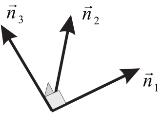
Thus, the set of eigenvectors can be used as an orthonormal basis.
Figure A.12: The orthonormal basis of eigenvectors { n ⃗ 1 , n ⃗ 2 , n ⃗ 3 } \{ \V{n}_1, \V{n}_2, \V{n}_3 \} { n 1 , n 2 , n 3 }
If a tensor A \T{A} A spectral form [17]
A = A ⋅ I = A ⋅ ( n ⃗ 1 n ⃗ 1 + n ⃗ 2 n ⃗ 2 + n ⃗ 3 n ⃗ 3 ) = λ 1 n ⃗ 1 n ⃗ 1 + λ 2 n ⃗ 2 n ⃗ 2 + λ 3 n ⃗ 3 n ⃗ 3 \begin{aligned}
\T{A} \;&=\; \T{A} \inp \T{I} \\
\;&=\; \T{A} \inp ( \V{n}_1\V{n}_1 + \V{n}_2\V{n}_2 + \V{n}_3\V{n}_3 ) \\
\;&=\; \lambda_1 \V{n}_1\V{n}_1 + \lambda_2 \V{n}_2\V{n}_2 + \lambda_3 \V{n}_3\V{n}_3
\end{aligned} A = A ⋅ I = A ⋅ ( n 1 n 1 + n 2 n 2 + n 3 n 3 ) = λ 1 n 1 n 1 + λ 2 n 2 n 2 + λ 3 n 3 n 3 The matrix A ‾ \M{A} A A \T{A} A
A ‾ = [ λ 1 0 0 0 λ 2 0 0 0 λ 3 ] \M{A} \;=\; \begin{bmatrix}
\lambda_1 & 0 & 0 \\
0 & \lambda_2 & 0 \\
0 & 0 & \lambda_3
\end{bmatrix} A = ⎣ ⎡ λ 1 0 0 0 λ 2 0 0 0 λ 3 ⎦ ⎤ Using the spectral form, some functions of a tensor can easily be calculated. E.g. for
the inverse , the square root , and the natural logarithm of a tensor
A \T{A} A
A − 1 = λ 1 − 1 n ⃗ 1 n ⃗ 1 + λ 2 − 1 n ⃗ 2 n ⃗ 2 + λ 3 − 1 n ⃗ 3 n ⃗ 3 A 1 / 2 = λ 1 1 / 2 n ⃗ 1 n ⃗ 1 + λ 2 1 / 2 n ⃗ 2 n ⃗ 2 + λ 3 1 / 2 n ⃗ 3 n ⃗ 3 ln A = ln ( λ 1 ) n ⃗ 1 n ⃗ 1 + ln ( λ 2 ) n ⃗ 2 n ⃗ 2 + ln ( λ 3 ) n ⃗ 3 n ⃗ 3 \begin{aligned}
\T{A}^{-1} \;&=\; \lambda_1^{-1} \V{n}_1\V{n}_1 + \lambda_2^{-1} \V{n}_2\V{n}_2 + \lambda_3^{-1} \V{n}_3\V{n}_3 \\
\T{A}^{1/2} \;&=\; \lambda_1^{1/2} \V{n}_1\V{n}_1 + \lambda_2^{1/2} \V{n}_2\V{n}_2 + \lambda_3^{1/2} \V{n}_3\V{n}_3 \\
\ln \T{A} \;&=\; \ln(\lambda_1) \V{n}_1\V{n}_1 + \ln(\lambda_2)
\V{n}_2\V{n}_2 + \ln(\lambda_3) \V{n}_3\V{n}_3
\end{aligned} A − 1 A 1/2 ln A = λ 1 − 1 n 1 n 1 + λ 2 − 1 n 2 n 2 + λ 3 − 1 n 3 n 3 = λ 1 1/2 n 1 n 1 + λ 2 1/2 n 2 n 2 + λ 3 1/2 n 3 n 3 = ln ( λ 1 ) n 1 n 1 + ln ( λ 2 ) n 2 n 2 + ln ( λ 3 ) n 3 n 3 A.3.6.4 Skewsymmetric tensor ¶ A tensor A \T{A} A skewsymmetric [18] antisymmetric if:
A T = − A \T{A}^T \;=\; - \T{A} A T = − A For the components A i j A_{ij} A ij A \T{A} A
A i j = − A j i ⇒ A i i = 0 A_{ij} \;=\; - A_{ji} \quad \Rightarrow \quad A_{ii} \;=\; 0 A ij = − A ji ⇒ A ii = 0 If A \T{A} A B \T{B} B
A : B = 0 e s p e c i a l l y A : I = tr A = 0 \T{A}:\T{B}=0 \quad {\rm especially} \quad \T{A}:\T{I} = \tr\T{A} = 0 A : B = 0 especially A : I = tr A = 0 The proof follows from:
A : B = A T : B T = − A : B \T{A} \dinp \T{B} \;=\; \T{A}^T \dinp \T{B}^T \;=\; - \T{A} \dinp \T{B} A : B = A T : B T = − A : B If A \T{A} A axial vector [19] ω ⃗ \V{\omega} ω
A ⋅ q ⃗ = ω ⃗ × q ⃗ \T{A} \inp \V{q} \;=\; \V{\omega} \cross \V{q} A ⋅ q = ω × q The proof of the existence of ω ⃗ \V{\omega} ω
A ⋅ q ⃗ = p ⃗ ⇒ q ⃗ ⋅ A ⋅ q ⃗ = q ⃗ ⋅ A T ⋅ q ⃗ = − q ⃗ ⋅ A ⋅ q ⃗ ⇒ q ⃗ ⋅ A ⋅ q ⃗ = 0 ⇒ q ⃗ ⋅ p ⃗ = 0 ⇒ q ⃗ ⊥ p ⃗ ⇒ ∃ ω ⃗ such that p ⃗ = ω ⃗ × q ⃗ \begin{aligned}
\T{A} \inp \V{q} \;&=\; \V{p} \quad \Rightarrow \\
\V{q} \inp \T{A} \inp \V{q} \;&=\; \V{q} \inp \T{A}^T \inp \V{q} \\
\;&=\; - \; \V{q} \inp \T{A} \inp \V{q} \quad \Rightarrow \\
\V{q} \inp \T{A} \inp \V{q} \;&=\; 0 \quad \Rightarrow \\
\V{q} \inp \V{p} \;&=\; 0 \quad \Rightarrow \\
\V{q} \;&\perp\; \V{p} \quad \Rightarrow \quad
\exists\;\V{\omega} \; \text{ such that } \V{p} \;=\; \V{\omega} \cross \V{q}
\end{aligned} A ⋅ q q ⋅ A ⋅ q q ⋅ A ⋅ q q ⋅ p q = p ⇒ = q ⋅ A T ⋅ q = − q ⋅ A ⋅ q ⇒ = 0 ⇒ = 0 ⇒ ⊥ p ⇒ ∃ ω such that p = ω × q On the other hand, if:
A ⋅ q ⃗ = ω ⃗ × q ⃗ ∀ q ⃗ \T{A} \inp \V{q} \;=\; \V{\omega} \cross \V{q} \quad \forall\ \V{q} A ⋅ q = ω × q ∀ q comparison of the following expressions:
A ⋅ q ⃗ = [ e ⃗ 1 e ⃗ 2 e ⃗ 3 ] [ A 11 A 12 A 13 A 21 A 22 A 23 A 31 A 32 A 33 ] [ q 1 q 2 q 3 ] = [ e ⃗ 1 e ⃗ 2 e ⃗ 3 ] [ A 11 q 1 + A 12 q 2 + A 13 q 3 A 21 q 1 + A 22 q 2 + A 23 q 3 A 31 q 1 + A 32 q 2 + A 33 q 3 ] \begin{aligned}
\T{A} \inp \V{q}
\;&=\;
\begin{bmatrix} \V{e}_1 & \V{e}_2 & \V{e}_3 \end{bmatrix}
\begin{bmatrix}
A_{11} & A_{12} & A_{13} \\
A_{21} & A_{22} & A_{23} \\
A_{31} & A_{32} & A_{33}
\end{bmatrix}
\begin{bmatrix} q_1 \\ q_2 \\ q_3 \end{bmatrix} \\
\;&=\;
\begin{bmatrix} \V{e}_1 & \V{e}_2 & \V{e}_3 \end{bmatrix}
\begin{bmatrix}
A_{11}q_1 + A_{12}q_2 + A_{13}q_3 \\
A_{21}q_1 + A_{22}q_2 + A_{23}q_3 \\
A_{31}q_1 + A_{32}q_2 + A_{33}q_3
\end{bmatrix}
\end{aligned} A ⋅ q = [ e 1 e 2 e 3 ] ⎣ ⎡ A 11 A 21 A 31 A 12 A 22 A 32 A 13 A 23 A 33 ⎦ ⎤ ⎣ ⎡ q 1 q 2 q 3 ⎦ ⎤ = [ e 1 e 2 e 3 ] ⎣ ⎡ A 11 q 1 + A 12 q 2 + A 13 q 3 A 21 q 1 + A 22 q 2 + A 23 q 3 A 31 q 1 + A 32 q 2 + A 33 q 3 ⎦ ⎤ and
ω ⃗ × q ⃗ = ( ω 1 e ⃗ 1 + ω 2 e ⃗ 2 + ω 3 e ⃗ 3 ) × ( q 1 e ⃗ 1 + q 2 e ⃗ 2 + q 3 e ⃗ 3 ) = ω 1 q 2 ( e ⃗ 3 ) + ω 1 q 3 ( − e ⃗ 2 ) + ω 2 q 1 ( − e ⃗ 3 ) + ω 2 q 3 ( e ⃗ 1 ) + ω 3 q 1 ( e ⃗ 2 ) + ω 3 q 2 ( − e ⃗ 1 ) = [ e ⃗ 1 e ⃗ 2 e ⃗ 3 ] [ ω 2 q 3 − ω 3 q 2 ω 3 q 1 − ω 1 q 3 ω 1 q 2 − ω 2 q 1 ] \begin{alignedat}{2}
\V{\omega} \cross \V{q}
\;&=\;
&&( \omega_1 \V{e}_1 + \omega_2 \V{e}_2 + \omega_3 \V{e}_3 ) \cross
( q_1 \V{e}_1 + q_2 \V{e}_2 + q_3 \V{e}_3 ) \\
\;&=\;
&&\omega_1 q_2 ( \V{e}_3) + \omega_1 q_3 (-\,\V{e}_2) +
\omega_2 q_1 (-\,\V{e}_3) + \omega_2 q_3 ( \V{e}_1) + \\
&&& \omega_3 q_1 ( \V{e}_2) + \omega_3 q_2 (-\,\V{e}_1) \\
\;&=\; && \begin{bmatrix} \V{e}_1 & \V{e}_2 & \V{e}_3 \end{bmatrix}
\begin{bmatrix}
\omega_2 q_3 - \omega_3 q_2 \\
\omega_3 q_1 - \omega_1 q_3 \\
\omega_1 q_2 - \omega_2 q_1
\end{bmatrix}
\end{alignedat} ω × q = = = ( ω 1 e 1 + ω 2 e 2 + ω 3 e 3 ) × ( q 1 e 1 + q 2 e 2 + q 3 e 3 ) ω 1 q 2 ( e 3 ) + ω 1 q 3 ( − e 2 ) + ω 2 q 1 ( − e 3 ) + ω 2 q 3 ( e 1 ) + ω 3 q 1 ( e 2 ) + ω 3 q 2 ( − e 1 ) [ e 1 e 2 e 3 ] ⎣ ⎡ ω 2 q 3 − ω 3 q 2 ω 3 q 1 − ω 1 q 3 ω 1 q 2 − ω 2 q 1 ⎦ ⎤ shows that:
A ‾ = [ 0 − ω 3 ω 2 ω 3 0 − ω 1 − ω 2 ω 1 0 ] \M{A} \;=\;
\begin{bmatrix}
0 & -\,\omega_3 & \omega_2 \\
\omega_3 & 0 & -\,\omega_1 \\
-\,\omega_2 & \omega_1 & 0
\end{bmatrix} A = ⎣ ⎡ 0 ω 3 − ω 2 − ω 3 0 ω 1 ω 2 − ω 1 0 ⎦ ⎤ and thus that the tensor A \T{A} A
A.3.6.5 Positive-definite tensor ¶ A tensor A \T{A} A positive-definite [20]
a ⃗ ⋅ A ⋅ a ⃗ > 0 ∀ a ⃗ ≠ 0 ⃗ \V{a} \inp \T{A} \inp \V{a} \;>\; 0 \quad \forall\;\V{a} \neq \V{0} a ⋅ A ⋅ a > 0 ∀ a = 0 A positive-definite tensor A \T{A} A
a ⃗ ⋅ A ⋅ a ⃗ = a ⃗ ⋅ A T ⋅ a ⃗ > 0 ∀ a ⃗ ≠ 0 ⃗ ⇒ a ⃗ ⋅ ( A − A T ) ⋅ a ⃗ = 0 ∧ a ⃗ ≠ 0 ⃗ \begin{aligned}
\V{a} \inp \T{A} \inp \V{a}
\;&=\; \V{a} \inp \T{A}^T \inp \V{a} \\
\;&>\; 0 \quad \forall\; \V{a} \neq \V{0} \quad \Rightarrow \\
\V{a} \inp (\T{A} - \T{A}^T) \inp \V{a} \;&=\; 0 \quad \wedge \quad \V{a} \neq \V{0}
\end{aligned} a ⋅ A ⋅ a a ⋅ ( A − A T ) ⋅ a = a ⋅ A T ⋅ a > 0 ∀ a = 0 ⇒ = 0 ∧ a = 0 If A \T{A} A A T = − A \T{A}^T = -\T{A} A T = − A
A.3.6.6 Orthogonal tensor ¶ A tensor A \T{A} A orthogonal [21]
( A ⋅ a ⃗ ) ⋅ ( A ⋅ b ⃗ ) = a ⃗ ⋅ b ⃗ ∀ a ⃗ , b ⃗ (\T{A} \inp \V{a}) \inp (\T{A} \inp \V{b}) \;=\; \V{a} \inp \V{b}
\quad \forall\ \V{a},\V{b} ( A ⋅ a ) ⋅ ( A ⋅ b ) = a ⋅ b ∀ a , b For the special case b ⃗ = a ⃗ \V{b} = \V{a} b = a
( A ⋅ a ⃗ ) ⋅ ( A ⋅ a ⃗ ) = a ⃗ ⋅ a ⃗ ⇒ ∥ A ⋅ a ⃗ ∥ = ∥ a ⃗ ∥ (\T{A} \inp \V{a}) \inp (\T{A} \inp \V{a}) \;=\; \V{a} \inp \V{a}
\quad \Rightarrow \quad \| \T{A} \inp \V{a} \| \;=\; \| \V{a} \| ( A ⋅ a ) ⋅ ( A ⋅ a ) = a ⋅ a ⇒ ∥ A ⋅ a ∥ = ∥ a ∥ Thus, an orthogonal transformation preserves lengths of vectors and
angles between vectors.
The inverse of an orthogonal tensor is identical to its conjugate:
A T = A − 1 \T{A}^T \;=\; \T{A}^{-1} A T = A − 1 as follows from:
( A ⋅ a ⃗ ) ⋅ ( A ⋅ b ⃗ ) = a ⃗ ⋅ A T ⋅ A ⋅ b ⃗ = a ⃗ ⋅ b ⃗ ⇒ A ⋅ A T = I ⇒ A T = A − 1 \begin{aligned}
(\T{A} \inp \V{a}) \inp (\T{A} \inp \V{b})
\;&=\; \V{a} \inp \T{A}^T \inp \T{A} \inp \V{b} \\
\;&=\; \V{a} \inp \V{b} \quad \Rightarrow \\
\T{A} \inp \T{A}^T \;&=\; \T{I} \quad \Rightarrow \\
\T{A}^T \;&=\; \T{A}^{-1}
\end{aligned} ( A ⋅ a ) ⋅ ( A ⋅ b ) A ⋅ A T A T = a ⋅ A T ⋅ A ⋅ b = a ⋅ b ⇒ = I ⇒ = A − 1 Moreover, this equation shows that:
det ( A ⋅ A T ) = [ det ( A ) ] 2 = det ( I ) = 1 ⇒ det ( A ) = ± 1 \begin{aligned}
\det(\T{A} \inp \T{A}^T) \;&=\; [\det(\T{A})]^2 = \det(\T{I}) = 1 \quad \Rightarrow \\
\det(\T{A}) \;&=\; \pm 1
\end{aligned} det ( A ⋅ A T ) det ( A ) = [ det ( A ) ] 2 = det ( I ) = 1 ⇒ = ± 1 Thus, an orthogonal tensor is a regular tensor. If det ( A ) = 1 \det(\T{A}) = 1 det ( A ) = 1 A \T{A} A rotation . If det ( A ) = − 1 \det(\T{A}) = -1 det ( A ) = − 1 A \T{A} A reflection .
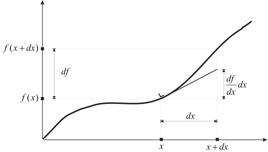
A.4 Spatial derivatives of scalar and vector fields ¶ A.4.1 Derivatives of functions of one or more variables ¶ Figure A.13: A function f f f x x x
Consider a scalar function f ( x ) f(x) f ( x ) x x x d f df df f f f d x dx d x x x x
d f = f ( x + d x ) − f ( x ) = f ( x ) + d f d x ∣ x d x + 1 2 d 2 f d x 2 ∣ x d x 2 + ⋯ − f ( x ) ≈ d f d x ∣ x d x \begin{aligned}
df \;&=\; f(x+dx) - f(x) \\
\;&=\; f(x) + \left.\tfrac{df}{dx}\right|_x dx +
\half \left.\tfrac{d^2f}{dx^2}\right|_x dx^2 + \dots - f(x) \\
\;&\approx\; \left.\tfrac{df}{dx}\right|_x dx
\end{aligned} df = f ( x + d x ) − f ( x ) = f ( x ) + d x df ∣ ∣ x d x + 2 1 d x 2 d 2 f ∣ ∣ x d x 2 + ⋯ − f ( x ) ≈ d x df ∣ ∣ x d x Extension to a function of two variables f ( x , y ) f(x,y) f ( x , y )
d f = f ( x + d x , y + d y ) − f ( x , y ) = f ( x , y ) + ∂ f ∂ x ∣ x , y d x + ∂ f ∂ y ∣ x , y d y + ⋯ − f ( x , y ) ≈ ∂ f ∂ x ∣ x , y d x + ∂ f ∂ y ∣ x , y d y \begin{aligned}
df \;&=\; f(x+dx,y+dy) - f(x,y) \\
\;&=\; f(x,y) + \left.\parder{f}{x}\right|_{x,y} dx +
\left.\parder{f}{y}\right|_{x,y} dy + \dots - f(x,y) \\
\;&\approx\; \left.\parder{f}{x}\right|_{x,y} dx +
\left.\parder{f}{y}\right|_{x,y} dy
\end{aligned} df = f ( x + d x , y + d y ) − f ( x , y ) = f ( x , y ) + ∂ x ∂ f ∣ ∣ x , y d x + ∂ y ∂ f ∣ ∣ x , y d y + ⋯ − f ( x , y ) ≈ ∂ x ∂ f ∣ ∣ x , y d x + ∂ y ∂ f ∣ ∣ x , y d y And for a function a ( x 1 , x 2 , x 3 ) a(x_1, x_2, x_3) a ( x 1 , x 2 , x 3 ) d a da d a a a a d x 1 dx_1 d x 1 d x 2 dx_2 d x 2 d x 3 dx_3 d x 3
d a = d x 1 ∂ a ∂ x 1 + d x 2 ∂ a ∂ x 2 + d x 3 ∂ a ∂ x 3 da \;=\; dx_1 \parder{a}{x_1} + dx_2 \parder{a}{x_2} + dx_3 \parder{a}{x_3} d a = d x 1 ∂ x 1 ∂ a + d x 2 ∂ x 2 ∂ a + d x 3 ∂ x 3 ∂ a The index notation for differentiation with respect to one of the
variables (i.c. x i x_i x i (A.106) d a da d a
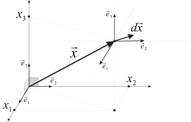
d a = d x i a , i da \;=\; dx_i a_{,i} d a = d x i a , i A.4.2 Components of the position vector ¶ In three-dimensional space, we may interpret the variables x 1 x_1 x 1 x 2 x_2 x 2 x 3 x_3 x 3 a ( x 1 , x 2 , x 3 ) a(x_1, x_2, x_3) a ( x 1 , x 2 , x 3 ) position
vector [22] x ⃗ \V{x} x { e ⃗ 1 , e ⃗ 2 , e ⃗ 3 } \basis { e 1 , e 2 , e 3 } x ⃗ \V{x} x origin O O O
x ⃗ = x 1 e ⃗ 1 + x 2 e ⃗ 2 + x 3 e ⃗ 3 \V{x} \;=\; x_1 \V{e}_1 + x_2 \V{e}_2 + x_3 \V{e}_3 x = x 1 e 1 + x 2 e 2 + x 3 e 3 Figure A.14: Components x i x_i x i x ⃗ \V{x} x { e ⃗ 1 , e ⃗ 2 , e ⃗ 3 } \basis { e 1 , e 2 , e 3 }
For the position vector x ⃗ + d x ⃗ \V{x} + d\V{x} x + d x
x ⃗ + d x ⃗ = ( x 1 + d x 1 ) e ⃗ 1 + ( x 2 + d x 2 ) e ⃗ 2 + ( x 3 + d x 3 ) e ⃗ 3 \V{x} + d\V{x} \;=\;
(x_1 + dx_1) \V{e}_1 + (x_2 + dx_2) \V{e}_2 + (x_3 + dx_3) \V{e}_3 x + d x = ( x 1 + d x 1 ) e 1 + ( x 2 + d x 2 ) e 2 + ( x 3 + d x 3 ) e 3 and thus the vector d x ⃗ d\V{x} d x
d x ⃗ = d x 1 e ⃗ 1 + d x 2 e ⃗ 2 + d x 3 e ⃗ 3 d\V{x} \;=\; dx_1 \V{e}_1 + dx_2 \V{e}_2 + dx_3 \V{e}_3 d x = d x 1 e 1 + d x 2 e 2 + d x 3 e 3 From the latter relation it is obvious that the changes d x 1 dx_1 d x 1 d x 2 dx_2 d x 2 d x 3 dx_3 d x 3 d x ⃗ d\V{x} d x
d x 1 = d x ⃗ ⋅ e ⃗ 1 d x 2 = d x ⃗ ⋅ e ⃗ 2 d x 3 = d x ⃗ ⋅ e ⃗ 3 \begin{aligned}
dx_1 \;&=\; d\V{x} \inp \V{e}_1 \\
dx_2 \;&=\; d\V{x} \inp \V{e}_2 \\
dx_3 \;&=\; d\V{x} \inp \V{e}_3
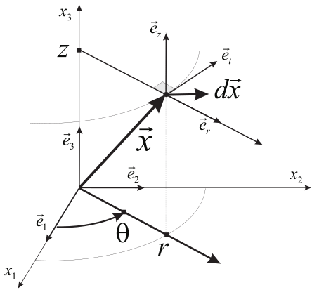
\end{aligned} d x 1 d x 2 d x 3 = d x ⋅ e 1 = d x ⋅ e 2 = d x ⋅ e 3 We could also express the function a ( x ⃗ ) a(\V{x}) a ( x ) r r r θ \theta θ z z z x ⃗ \V{x} x { e ⃗ r , e ⃗ t , e ⃗ z } \cylbasis { e r , e t , e z }
x ⃗ = r e ⃗ r ( θ ) + z e ⃗ z \V{x} \;=\; r \V{e}_r(\theta) + z \V{e}_z x = r e r ( θ ) + z e z Figure A.15: Components r r r θ \theta θ z z z x ⃗ \V{x} x { e ⃗ r , e ⃗ t , e ⃗ z } \cylbasis { e r , e t , e z }
Within the cylindrical basis, the position x ⃗ + d x ⃗ \V{x} + d\V{x} x + d x
x ⃗ + d x ⃗ = ( r + d r ) e ⃗ r ( θ + d θ ) + ( z + d z ) e ⃗ z = ( r + d r ) { e ⃗ r ( θ ) + d e ⃗ r d θ d θ } + ( z + d z ) e ⃗ z = r e ⃗ r ( θ ) + z e ⃗ z + r e ⃗ t ( θ ) d θ + d r e ⃗ r ( θ ) + e ⃗ t ( θ ) d r d θ + d z e ⃗ z \begin{alignedat}{2}
\V{x} + d\V{x}
\;&=\; &&(r + dr) \V{e}_r(\theta + d\theta) + (z + dz) \V{e}_z \\
\;&=\; &&(r + dr) \{ \V{e}_r(\theta) + \tfrac{d\V{e}_r}{d\theta} d\theta \} +
(z + dz) \V{e}_z \\
\;&=\; &&r \V{e}_r(\theta) + z \V{e}_z + \\
& &&r \V{e}_t(\theta) d\theta +
dr \V{e}_r(\theta) + \V{e}_t(\theta) dr d\theta + dz \V{e}_z
\end{alignedat} x + d x = = = ( r + d r ) e r ( θ + d θ ) + ( z + d z ) e z ( r + d r ) { e r ( θ ) + d θ d e r d θ } + ( z + d z ) e z r e r ( θ ) + z e z + r e t ( θ ) d θ + d r e r ( θ ) + e t ( θ ) d r d θ + d z e z from which it can be concluded that, in a linear approximation, the
vector d x ⃗ d\V{x} d x
d x ⃗ ≈ d r e ⃗ r ( θ ) + r d θ e ⃗ t ( θ ) + d z e ⃗ z d\V{x} \;\approx\; dr \V{e}_r(\theta) + r d\theta \V{e}_t(\theta) + dz
\V{e}_z d x ≈ d r e r ( θ ) + r d θ e t ( θ ) + d z e z The changes d r dr d r d θ d\theta d θ d z dz d z d x ⃗ d\V{x} d x
d r = d x ⃗ ⋅ e ⃗ r d θ = 1 r d x ⃗ ⋅ e ⃗ t d z = d x ⃗ ⋅ e ⃗ z \begin{aligned}
dr \;&=\; d\V{x} \inp \V{e}_r \\
d\theta \;&=\; \tfrac{1}{r} d\V{x} \inp \V{e}_t\\
dz \;&=\; d\V{x} \inp \V{e}_z
\end{aligned} d r d θ d z = d x ⋅ e r = r 1 d x ⋅ e t = d x ⋅ e z A.4.3 The gradient operator ¶ Considering a a a x ⃗ \V{x} x d a da d a d x ⃗ d\V{x} d x
d a = d x 1 ∂ a ∂ x 1 + d x 2 ∂ a ∂ x 2 + d x 3 ∂ a ∂ x 3 = ( d x ⃗ ⋅ e ⃗ 1 ) ∂ a ∂ x 1 + ( d x ⃗ ⋅ e ⃗ 2 ) ∂ a ∂ x 2 + ( d x ⃗ ⋅ e ⃗ 3 ) ∂ a ∂ x 3 = d x ⃗ ⋅ [ e ⃗ 1 ∂ a ∂ x 1 + e ⃗ 2 ∂ a ∂ x 2 + e ⃗ 3 ∂ a ∂ x 3 ] = d x ⃗ ⋅ ( ∇ ⃗ a ) \begin{aligned}
da \;&=\; dx_1 \parder{a}{x_1} + dx_2 \parder{a}{x_2} + dx_3 \parder{a}{x_3} \\
\;&=\; (d\V{x} \inp \V{e}_1) \parder{a}{x_1} + (d\V{x} \inp \V{e}_2) \parder{a}{x_2} +
(d\V{x} \inp \V{e}_3) \parder{a}{x_3} \\
\;&=\; d\V{x} \inp \left[ \V{e}_1 \parder{a}{x_1} + \V{e}_2 \parder{a}{x_2} +
\V{e}_3 \parder{a}{x_3} \right] \\
\;&=\; d\V{x} \inp (\grad a)
\end{aligned} d a = d x 1 ∂ x 1 ∂ a + d x 2 ∂ x 2 ∂ a + d x 3 ∂ x 3 ∂ a = ( d x ⋅ e 1 ) ∂ x 1 ∂ a + ( d x ⋅ e 2 ) ∂ x 2 ∂ a + ( d x ⋅ e 3 ) ∂ x 3 ∂ a = d x ⋅ [ e 1 ∂ x 1 ∂ a + e 2 ∂ x 2 ∂ a + e 3 ∂ x 3 ∂ a ] = d x ⋅ ( ∇ a ) The symbol ∇ ⃗ \grad ∇ gradient operator [23]
∇ ⃗ = [ e ⃗ 1 ∂ ∂ x 1 + e ⃗ 2 ∂ ∂ x 2 + e ⃗ 3 ∂ ∂ x 3 ] = e ⃗ ∼ T ∇ ∼ \begin{aligned}
\grad \;&=\; \left[ \V{e}_1 \parder{}{x_1} + \V{e}_2 \parder{}{x_2} +
\V{e}_3 \parder{}{x_3} \right] \\
\;&=\; \C{\V{e}}^T \C{\nabla}
\end{aligned} ∇ = [ e 1 ∂ x 1 ∂ + e 2 ∂ x 2 ∂ + e 3 ∂ x 3 ∂ ] = ∼ e T ∼ ∇ and
the expression ∇ ⃗ a \grad a ∇ a gradient of a a a a ⃗ \V{a} a
d a ⃗ = d x 1 ∂ a ⃗ ∂ x 1 + d x 2 ∂ a ⃗ ∂ x 2 + d x 3 ∂ a ⃗ ∂ x 3 = ( d x ⃗ ⋅ e ⃗ 1 ) ∂ a ⃗ ∂ x 1 + ( d x ⃗ ⋅ e ⃗ 2 ) ∂ a ⃗ ∂ x 2 + ( d x ⃗ ⋅ e ⃗ 3 ) ∂ a ⃗ ∂ x 3 = d x ⃗ ⋅ [ e ⃗ 1 ∂ a ⃗ ∂ x 1 + e ⃗ 2 ∂ a ⃗ ∂ x 2 + e ⃗ 3 ∂ a ⃗ ∂ x 3 ] = d x ⃗ ⋅ ( ∇ ⃗ a ⃗ ) \begin{aligned}
d\V{a} \;&=\; dx_1 \parder{\V{a}}{x_1} + dx_2 \parder{\V{a}}{x_2} + dx_3 \parder{\V{a}}{x_3} \\
\;&=\; (d\V{x} \inp \V{e}_1) \parder{\V{a}}{x_1} +
(d\V{x} \inp \V{e}_2) \parder{\V{a}}{x_2} +
(d\V{x} \inp \V{e}_3) \parder{\V{a}}{x_3} \\
\;&=\; d\V{x} \inp \left[ \V{e}_1 \parder{\V{a}}{x_1} + \V{e}_2 \parder{\V{a}}{x_2} +
\V{e}_3 \parder{\V{a}}{x_3} \right] \\
\;&=\; d\V{x} \inp (\grad \V{a})
\end{aligned} d a = d x 1 ∂ x 1 ∂ a + d x 2 ∂ x 2 ∂ a + d x 3 ∂ x 3 ∂ a = ( d x ⋅ e 1 ) ∂ x 1 ∂ a + ( d x ⋅ e 2 ) ∂ x 2 ∂ a + ( d x ⋅ e 3 ) ∂ x 3 ∂ a = d x ⋅ [ e 1 ∂ x 1 ∂ a + e 2 ∂ x 2 ∂ a + e 3 ∂ x 3 ∂ a ] = d x ⋅ ( ∇ a ) or in index notation
d a j = d x i a j , i da_j \;=\; dx_i a_{j,i} d a j = d x i a j , i For the special case a ⃗ = x ⃗ \V{a} = \V{x} a = x
∇ ⃗ x ⃗ = I \grad \V{x} \;=\; \T{I} ∇ x = I The gradient operator ∇ ⃗ \grad ∇ a ⃗ \V{a} a gradient of a ⃗ \V{a} a a ⃗ \V{a} a divergence [24] a ⃗ \V{a} a a ⃗ \V{a} a rotation [25] curl of a ⃗ \V{a} a a ⃗ \V{a} a
g r a d a ⃗ = ∇ ⃗ a ⃗ = e ⃗ 1 ∂ a ⃗ ∂ x 1 + e ⃗ 2 ∂ a ⃗ ∂ x 2 + e ⃗ 3 ∂ a ⃗ ∂ x 3 , d i v a ⃗ = ∇ ⃗ ⋅ a ⃗ = e ⃗ 1 ⋅ ∂ a ⃗ ∂ x 1 + e ⃗ 2 ⋅ ∂ a ⃗ ∂ x 2 + e ⃗ 3 ⋅ ∂ a ⃗ ∂ x 3 , r o t a ⃗ = ∇ ⃗ × a ⃗ = e ⃗ 1 × ∂ a ⃗ ∂ x 1 + e ⃗ 2 × ∂ a ⃗ ∂ x 2 + e ⃗ 3 × ∂ a ⃗ ∂ x 3 \begin{aligned}
{\rm grad\ }\V{a} \;&=\; \grad \V{a}
= \V{e}_1 \parder{\V{a}}{x_1} + \V{e}_2 \parder{\V{a}}{x_2} +
\V{e}_3 \parder{\V{a}}{x_3} ,\\
{\rm div\ }\V{a} \;&=\; \grad \inp \V{a}
= \V{e}_1 \inp \parder{\V{a}}{x_1} + \V{e}_2 \inp \parder{\V{a}}{x_2} +
\V{e}_3 \inp \parder{\V{a}}{x_3} ,\\
{\rm rot\ }\V{a} \;&=\; \grad \cross \V{a}
= \V{e}_1 \cross \parder{\V{a}}{x_1} + \V{e}_2 \cross \parder{\V{a}}{x_2} +
\V{e}_3 \cross \parder{\V{a}}{x_3}
\end{aligned} grad a div a rot a = ∇ a = e 1 ∂ x 1 ∂ a + e 2 ∂ x 2 ∂ a + e 3 ∂ x 3 ∂ a , = ∇ ⋅ a = e 1 ⋅ ∂ x 1 ∂ a + e 2 ⋅ ∂ x 2 ∂ a + e 3 ⋅ ∂ x 3 ∂ a , = ∇ × a = e 1 × ∂ x 1 ∂ a + e 2 × ∂ x 2 ∂ a + e 3 × ∂ x 3 ∂ a Note that div a ⃗ \V{a} a a ⃗ \V{a} a a ⃗ \V{a} a
The expression for the gradient operator in cylindrical coordinates can be found
following a similar derivation as in the case of a Cartesian coordinate
system:
d a = d r ∂ a ∂ r + d θ ∂ a ∂ θ + d z ∂ a ∂ z = ( d x ⃗ ⋅ e ⃗ r ) ∂ a ∂ r + ( 1 r d x ⃗ ⋅ e ⃗ t ) ∂ a ∂ θ + ( d x ⃗ ⋅ e ⃗ z ) ∂ a ∂ z = d x ⃗ ⋅ [ e ⃗ r ∂ a ∂ r + 1 r e ⃗ t ∂ a ∂ θ + e ⃗ z ∂ a ∂ z ] = d x ⃗ ⋅ ( ∇ ⃗ a ) \begin{aligned}
da \;&=\; dr \parder{a}{r} + d\theta \parder{a}{\theta} + dz \parder{a}{z} \\
\;&=\; (d\V{x} \inp \V{e}_r) \parder{a}{r} +
(\tfrac{1}{r} d\V{x} \inp \V{e}_t) \parder{a}{\theta} +
(d\V{x} \inp \V{e}_z) \parder{a}{z} \\
\;&=\; d\V{x} \inp \left[ \V{e}_r \parder{a}{r} +
\tfrac{1}{r} \V{e}_t \parder{a}{\theta} + \V{e}_z \parder{a}{z} \right] \\
\;&=\; d\V{x} \inp (\grad a)
\end{aligned} d a = d r ∂ r ∂ a + d θ ∂ θ ∂ a + d z ∂ z ∂ a = ( d x ⋅ e r ) ∂ r ∂ a + ( r 1 d x ⋅ e t ) ∂ θ ∂ a + ( d x ⋅ e z ) ∂ z ∂ a = d x ⋅ [ e r ∂ r ∂ a + r 1 e t ∂ θ ∂ a + e z ∂ z ∂ a ] = d x ⋅ ( ∇ a ) Thus the expression for the gradient operator
in a cylindrical coordinate system equals:
∇ ⃗ = e ⃗ r ∂ ∂ r + e ⃗ t 1 r ∂ ∂ θ + e ⃗ z ∂ ∂ z \grad \;=\;
\V{e}_r \parder{}{r} + \V{e}_t \frac{1}{r} \parder{}{\theta} + \V{e}_z \parder{}{z} ∇ = e r ∂ r ∂ + e t r 1 ∂ θ ∂ + e z ∂ z ∂ The following relations on differentiable scalar functions ϕ \phi ϕ a ⃗ , b ⃗ \V{a},\V{b} a , b A , B , C \T{A},\T{B},\T{C} A , B , C
A : ( B ⋅ C ) = ( A ⋅ B ) : C ∇ ⃗ ( ϕ a ⃗ ) = ( ∇ ⃗ ϕ ) a ⃗ + ϕ ∇ ⃗ a ⃗ ∇ ⃗ ⋅ ( ϕ a ⃗ ) = ( ∇ ⃗ ϕ ) ⋅ a ⃗ + ϕ ∇ ⃗ ⋅ a ⃗ ∇ ⃗ ( a ⃗ ⋅ b ⃗ ) = ( ∇ ⃗ a ⃗ ) ⋅ b ⃗ + ( ∇ ⃗ b ⃗ ) ⋅ a ⃗ ∇ ⃗ ⋅ ( a ⃗ b ⃗ ) = ( ∇ ⃗ ⋅ a ⃗ ) b ⃗ + a ⃗ ⋅ ∇ ⃗ b ⃗ ∇ ⃗ ⋅ ( ϕ A ) = ( ∇ ⃗ ϕ ) ⋅ A + ϕ ∇ ⃗ ⋅ A ∇ ⃗ ⋅ ( A ⋅ a ⃗ ) = ( ∇ ⃗ ⋅ A ) ⋅ a ⃗ + A : ( ∇ ⃗ a ⃗ ) T ∇ ⃗ ⋅ a ⃗ = ( ∇ ⃗ a ⃗ ) : I = tr ( ∇ ⃗ a ⃗ ) \begin{aligned}
\T{A} \dinp (\T{B}\inp\T{C}) \;&=\; (\T{A}\inp\T{B}) \dinp \T{C}\\
\grad(\phi\V{a}) \;&=\; (\grad\phi)\V{a} + \phi\grad\V{a}\\
\grad \inp (\phi \V{a}) \;&=\; (\grad\phi) \inp \V{a} + \phi \grad \inp \V{a}\\
\grad(\V{a}\inp\V{b}) \;&=\; (\grad\V{a})\inp\V{b} + (\grad\V{b})\inp\V{a}\\
\grad \inp (\V{a}\V{b}) \;&=\; (\grad \inp \V{a}) \V{b} + \V{a} \inp \grad\V{b}\\
\grad \inp (\phi \T{A}) \;&=\; (\grad\phi) \inp \T{A} + \phi \grad \inp \T{A}\\
\grad \inp (\T{A} \inp \V{a}) \;&=\; (\grad \inp \T{A}) \inp \V{a} + \T{A} :(\grad\V{a})^T\\
\grad \inp \V{a} \;&=\; (\grad\V{a}) \dinp \T{I} = \tr(\grad\V{a})
\end{aligned} A : ( B ⋅ C ) ∇ ( ϕ a ) ∇ ⋅ ( ϕ a ) ∇ ( a ⋅ b ) ∇ ⋅ ( a b ) ∇ ⋅ ( ϕ A ) ∇ ⋅ ( A ⋅ a ) ∇ ⋅ a = ( A ⋅ B ) : C = ( ∇ ϕ ) a + ϕ ∇ a = ( ∇ ϕ ) ⋅ a + ϕ ∇ ⋅ a = ( ∇ a ) ⋅ b + ( ∇ b ) ⋅ a = ( ∇ ⋅ a ) b + a ⋅ ∇ b = ( ∇ ϕ ) ⋅ A + ϕ ∇ ⋅ A = ( ∇ ⋅ A ) ⋅ a + A : ( ∇ a ) T = ( ∇ a ) : I = tr ( ∇ a ) A.6 Gauss’ divergence theorem ¶ Gauss’ divergence theorem relates volume integrals and surface integrals.
Let’s consider a closed volume V V V A A A n ⃗ \vec{n} n a ⃗ \vec{a} a V V V V V V p ⃗ \vec{p} p A A A p ⃗ \vec{p} p
∫ ∫ ∫ V ∇ ⃗ ⋅ p ⃗ d V = ∫ ∫ A n ⃗ ⋅ p ⃗ d A = ∫ ∫ A p ⃗ ⋅ n ⃗ d A \int\int\int_V \: \grad \inp \vec{p} \: dV \;=\; \int\int_A \: \vec{n} \inp \vec{p} \: dA \;=\; \int\int_A \: \vec{p}\inp\vec{n} \: dA ∫∫ ∫ V ∇ ⋅ p d V = ∫ ∫ A n ⋅ p d A = ∫ ∫ A p ⋅ n d A The divergence theorem is often used in deriving balance equations in continua.
Using the divergence theorem, it is often possible to convert volume integrals into surface integrals, if a vector field can be found of which the divergence equals the integrand in the volume integral.
The generalised form of Gauss’ divergence theorem applies to a tensor field P \T{P} P
∫ ∫ ∫ V ∇ ⃗ ⋅ P d V = ∫ ∫ A n ⃗ ⋅ P d A \int\int\int_V \: \grad \inp \T{P} \: dV \;=\; \int\int_A \: \vec{n} \inp \T{P} \: dA ∫∫ ∫ V ∇ ⋅ P d V = ∫ ∫ A n ⋅ P d A A.7 Higher-order and fourth-order tensors ¶ A.7.1 Definition ¶ Some problems invoke the transformation of tensors. Such transformations are carried out
by means of higher-order tensors. A general definition of a tensor could be: an
invariant object with an arbitrary number of indices . The number of indices is the
order (or rank) of the tensor. The transformation which is most relevant in the
mechanics of materials is the transformation of a second-order tensor into another
second-order tensor by means of a fourth-order tensor.
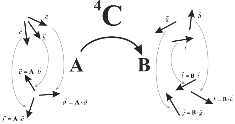
Figure A.16: A fourth-order tensor 4 C \TQ{C} 4 C A \T{A} A B \T{B} B
An arbitrary tensor A \T{A} A B \T{B} B 4 C \TQ{C} 4 C Figure A.16
B = 4 C : A \T{B} \;=\; \TQ{C} \dinp \T{A} B = 4 C : A Using index tensor notations, the tensor A l k A_{lk} A l k B i j B_{ij} B ij
B i j = C i j k l A l k B_{ij} \;=\; C_{ijkl}\,A_{lk} B ij = C ijk l A l k The tensor C i j k l C_{ijkl} C ijk l
A.7.2 Properties ¶ Since a fourth-order tensor is built on quadrades rather than dyades, some new calculus
rules apply. Each fourth-order tensor can be written as a finite sum of quadrades. With
respect to a two-dimensional Cartesian basis, a tensor 4 C \TQ{C} 4 C s i x t e e n sixteen s i x t ee n
4 C = C 1111 e ⃗ 1 e ⃗ 1 e ⃗ 1 e ⃗ 1 + C 1112 e ⃗ 1 e ⃗ 1 e ⃗ 1 e ⃗ 2 + C 1121 e ⃗ 1 e ⃗ 1 e ⃗ 2 e ⃗ 1 + C 1122 e ⃗ 1 e ⃗ 1 e ⃗ 2 e ⃗ 2 C 1211 e ⃗ 1 e ⃗ 2 e ⃗ 1 e ⃗ 1 + C 1212 e ⃗ 1 e ⃗ 2 e ⃗ 1 e ⃗ 2 + C 1221 e ⃗ 1 e ⃗ 2 e ⃗ 2 e ⃗ 1 + C 1222 e ⃗ 1 e ⃗ 2 e ⃗ 2 e ⃗ 2 C 2111 e ⃗ 2 e ⃗ 1 e ⃗ 1 e ⃗ 1 + C 2112 e ⃗ 2 e ⃗ 1 e ⃗ 1 e ⃗ 2 + C 2121 e ⃗ 2 e ⃗ 1 e ⃗ 2 e ⃗ 1 + C 2122 e ⃗ 2 e ⃗ 1 e ⃗ 2 e ⃗ 2 C 2211 e ⃗ 2 e ⃗ 2 e ⃗ 1 e ⃗ 1 + C 2212 e ⃗ 2 e ⃗ 2 e ⃗ 1 e ⃗ 2 + C 2221 e ⃗ 2 e ⃗ 2 e ⃗ 2 e ⃗ 1 + C 2222 e ⃗ 2 e ⃗ 2 e ⃗ 2 e ⃗ 2 \begin{split}
\TQ{C} \;=\; & C_{1111}\V{e}_1\V{e}_1\V{e}_1\V{e}_1 +
C_{1112}\V{e}_1\V{e}_1\V{e}_1\V{e}_2 + C_{1121}\V{e}_1\V{e}_1\V{e}_2\V{e}_1 + C_{1122}\V{e}_1\V{e}_1\V{e}_2\V{e}_2\\
& C_{1211}\V{e}_1\V{e}_2\V{e}_1\V{e}_1 +
C_{1212}\V{e}_1\V{e}_2\V{e}_1\V{e}_2 + C_{1221}\V{e}_1\V{e}_2\V{e}_2\V{e}_1 +
C_{1222}\V{e}_1\V{e}_2\V{e}_2\V{e}_2\\
& C_{2111}\V{e}_2\V{e}_1\V{e}_1\V{e}_1 +
C_{2112}\V{e}_2\V{e}_1\V{e}_1\V{e}_2 + C_{2121}\V{e}_2\V{e}_1\V{e}_2\V{e}_1 +
C_{2122}\V{e}_2\V{e}_1\V{e}_2\V{e}_2\\
& C_{2211}\V{e}_2\V{e}_2\V{e}_1\V{e}_1 +
C_{2212}\V{e}_2\V{e}_2\V{e}_1\V{e}_2 + C_{2221}\V{e}_2\V{e}_2\V{e}_2\V{e}_1 + C_{2222}\V{e}_2\V{e}_2\V{e}_2\V{e}_2
\end{split} 4 C = C 1111 e 1 e 1 e 1 e 1 + C 1112 e 1 e 1 e 1 e 2 + C 1121 e 1 e 1 e 2 e 1 + C 1122 e 1 e 1 e 2 e 2 C 1211 e 1 e 2 e 1 e 1 + C 1212 e 1 e 2 e 1 e 2 + C 1221 e 1 e 2 e 2 e 1 + C 1222 e 1 e 2 e 2 e 2 C 2111 e 2 e 1 e 1 e 1 + C 2112 e 2 e 1 e 1 e 2 + C 2121 e 2 e 1 e 2 e 1 + C 2122 e 2 e 1 e 2 e 2 C 2211 e 2 e 2 e 1 e 1 + C 2212 e 2 e 2 e 1 e 2 + C 2221 e 2 e 2 e 2 e 1 + C 2222 e 2 e 2 e 2 e 2 In a three-dimensional space a tensor 4 C \TQ{C} 4 C 3 × 3 × 3 × 3 = 81 3 \times\ 3 \times 3 \times 3 = 81 3 × 3 × 3 × 3 = 81 [ 3 × 3 × 3 × 3 ] [3 \times 3 \times 3 \times 3] [ 3 × 3 × 3 × 3 ]
Different types of transposed tensors are defined: the total transpose 4 C T \TQ{C}^{T} 4 C T 4 C L T \TQ{C}^{LT} 4 C L T 4 C R T \TQ{C}^{RT} 4 C RT 4 C \TQ{C} 4 C C i j k l C_{ijkl} C ijk l
4 C T ⇔ C l k j i 4 C L T ⇔ C j i k l 4 C R T ⇔ C i j l k \begin{aligned}
\TQ{C}^{T} \;&\Leftrightarrow\; C_{lkji} \\
\TQ{C}^{LT} \;&\Leftrightarrow\; C_{jikl} \\
\TQ{C}^{RT} \;&\Leftrightarrow\; C_{ijlk}
\end{aligned} 4 C T 4 C L T 4 C RT ⇔ C l kji ⇔ C jik l ⇔ C ij l k Different types of minor symmetries can be defined for a fourth-order tensor.
A left symmetric fourth-order tensor, is a tensor for which
4 C = 4 C L T ⟹ C i j k l = C j i k l \TQ{C} \;=\;\TQ{C}^{LT} \quad\Longrightarrow\quad C_{ijkl}\;=\;C_{jikl} 4 C = 4 C L T ⟹ C ijk l = C jik l In a 3D space, it has 81 − 1 × 3 × 3 × 3 = 54 81 - 1 \times 3 \times 3 \times 3 = 54 81 − 1 × 3 × 3 × 3 = 54 right symmetric fourth-order tensor is given by
4 C = 4 C R T ⟹ C i j k l = C i j l k \TQ{C} \;=\;\TQ{C}^{RT} \quad\Longrightarrow\quad C_{ijkl}\;=\;C_{ijlk} 4 C = 4 C RT ⟹ C ijk l = C ij l k In a 3D space, it has 81 − 3 × 3 × 3 × 1 = 54 81 - 3 \times 3 \times 3 \times 1 = 54 81 − 3 × 3 × 3 × 1 = 54 54 − 1 × 3 × 3 × 2 = 36 54 - 1 \times 3 \times 3 \times 2 = 36 54 − 1 × 3 × 3 × 2 = 36 middle symmetric fourth-order tensor complies with
4 C = 4 C T ⟹ C i j k l = C l k j i \TQ{C} \;=\;\TQ{C}^{T} \quad\Longrightarrow\quad C_{ijkl}\;=\;C_{lkji} 4 C = 4 C T ⟹ C ijk l = C l kji In a 3D space, it has 81 − 2 × 3 × 3 × 2 = 45 81 - 2 \times 3 \times 3 \times 2 = 45 81 − 2 × 3 × 3 × 2 = 45 total symmetric fourth-order tensor equals is left, right and
central symmetric, i.e.
4 C = 4 C L T = 4 C R T = 4 C T \TQ{C} \;=\; \TQ{C}^{LT} \;=\; \TQ{C}^{RT} \;=\; \TQ{C}^{T} 4 C = 4 C L T = 4 C RT = 4 C T In a 3D space, it has 36 − 1 2 6 × 5 = 21 36 - \half 6 \times 5 = 21 36 − 2 1 6 × 5 = 21
The fourth-order null tensor 4 0 \TQ{0} 4 0
4 0 : A = 0 \TQ{0}\dinp\T{A} \;=\; \T{0} 4 0 : A = 0 The fourth-order unit tensor 4 I \TQ{I} 4 I A \T{A} A
4 I : A = A \TQ{I}\dinp\T{A} \;=\; \T{A} 4 I : A = A This tensor is given in index notation by
4 I ⟹ I i j k l = δ i l δ j k \TQ{I} \;\Longrightarrow\; I_{ijkl} \;=\; \delta_{il}\delta_{jk} 4 I ⟹ I ijk l = δ i l δ jk or with respect to a 3D Cartesian basis
4 I = e ⃗ 1 e ⃗ 1 e ⃗ 1 e ⃗ 1 + e ⃗ 1 e ⃗ 2 e ⃗ 2 e ⃗ 1 + e ⃗ 1 e ⃗ 3 e ⃗ 3 e ⃗ 1 e ⃗ 2 e ⃗ 1 e ⃗ 1 e ⃗ 2 + e ⃗ 2 e ⃗ 2 e ⃗ 2 e ⃗ 2 + e ⃗ 2 e ⃗ 3 e ⃗ 3 e ⃗ 2 e ⃗ 3 e ⃗ 1 e ⃗ 1 e ⃗ 3 + e ⃗ 3 e ⃗ 2 e ⃗ 2 e ⃗ 3 + e ⃗ 3 e ⃗ 3 e ⃗ 3 e ⃗ 3 \begin{split}
\TQ{I} \;=\; &\V{e}_1\V{e}_1\V{e}_1\V{e}_1 + \V{e}_1\V{e}_2\V{e}_2\V{e}_1 +
\V{e}_1\V{e}_3\V{e}_3\V{e}_1 \\
&\V{e}_2\V{e}_1\V{e}_1\V{e}_2 + \V{e}_2\V{e}_2\V{e}_2\V{e}_2 +
\V{e}_2\V{e}_3\V{e}_3\V{e}_2 \\
&\V{e}_3\V{e}_1\V{e}_1\V{e}_3 + \V{e}_3\V{e}_2\V{e}_2\V{e}_3 +
\V{e}_3\V{e}_3\V{e}_3\V{e}_3
\end{split} 4 I = e 1 e 1 e 1 e 1 + e 1 e 2 e 2 e 1 + e 1 e 3 e 3 e 1 e 2 e 1 e 1 e 2 + e 2 e 2 e 2 e 2 + e 2 e 3 e 3 e 2 e 3 e 1 e 1 e 3 + e 3 e 2 e 2 e 3 + e 3 e 3 e 3 e 3 The symmetric fourth-order unit tensor 4 I s \TQ{I}^s 4 I s A \T{A} A A \T{A} A A s \T{A}^s A s
4 I s : A = A s = 1 2 ( A + A T ) \TQ{I}^s\dinp\T{A} \;=\; \T{A}^s \;=\; \tfrac{1}{2}(\T{A} + \T{A}^T) 4 I s : A = A s = 2 1 ( A + A T ) This tensor is given in index notation by
4 I s ⇔ I i j k l s = 1 2 ( δ i l δ j k + δ i k δ j l ) \TQ{I}^s \;\Leftrightarrow\; I_{ijkl}^s \;=\; \tfrac{1}{2}\left(\delta_{il}\delta_{jk} + \delta_{ik}\delta_{jl}\right) 4 I s ⇔ I ijk l s = 2 1 ( δ i l δ jk + δ ik δ j l ) This tensor is a total symmetric tensor, i.e. left symmetric, right symmetric and central symmetric.
Note that this tensor is also given by
4 I s = 1 2 ( 4 I + 4 I R T ) \TQ{I}^s \;=\; \tfrac{1}{2}(\TQ{I}+\TQ{I}^{RT}) 4 I s = 2 1 ( 4 I + 4 I RT ) or with respect to a Cartesian basis by
4 I s = e ⃗ 1 e ⃗ 1 e ⃗ 1 e ⃗ 1 + 1 2 e ⃗ 1 e ⃗ 2 e ⃗ 2 e ⃗ 1 + 1 2 e ⃗ 1 e ⃗ 2 e ⃗ 1 e ⃗ 2 + 1 2 e ⃗ 1 e ⃗ 3 e ⃗ 3 e ⃗ 1 + 1 2 e ⃗ 1 e ⃗ 3 e ⃗ 1 e ⃗ 3 1 2 e ⃗ 2 e ⃗ 1 e ⃗ 1 e ⃗ 2 + 1 2 e ⃗ 2 e ⃗ 1 e ⃗ 2 e ⃗ 1 + e ⃗ 2 e ⃗ 2 e ⃗ 2 e ⃗ 2 + 1 2 e ⃗ 2 e ⃗ 3 e ⃗ 3 e ⃗ 2 + 1 2 e ⃗ 2 e ⃗ 3 e ⃗ 2 e ⃗ 3 1 2 e ⃗ 3 e ⃗ 1 e ⃗ 1 e ⃗ 3 + 1 2 e ⃗ 3 e ⃗ 1 e ⃗ 3 e ⃗ 1 + 1 2 e ⃗ 3 e ⃗ 2 e ⃗ 2 e ⃗ 3 + 1 2 e ⃗ 3 e ⃗ 2 e ⃗ 3 e ⃗ 2 + e ⃗ 3 e ⃗ 3 e ⃗ 3 e ⃗ 3 \begin{split}
\TQ{I}^s \;=\; &\V{e}_1\V{e}_1\V{e}_1\V{e}_1 + \tfrac{1}{2}\V{e}_1\V{e}_2\V{e}_2\V{e}_1 +
\tfrac{1}{2}\V{e}_1\V{e}_2\V{e}_1\V{e}_2 + \tfrac{1}{2}\V{e}_1\V{e}_3\V{e}_3\V{e}_1
+ \tfrac{1}{2}\V{e}_1\V{e}_3\V{e}_1\V{e}_3 \\
& \tfrac{1}{2}\V{e}_2\V{e}_1\V{e}_1\V{e}_2 + \tfrac{1}{2}\V{e}_2\V{e}_1\V{e}_2\V{e}_1 +
\V{e}_2\V{e}_2\V{e}_2\V{e}_2 + \tfrac{1}{2}\V{e}_2\V{e}_3\V{e}_3\V{e}_2 +
\tfrac{1}{2}\V{e}_2\V{e}_3\V{e}_2\V{e}_3 \\
& \tfrac{1}{2}\V{e}_3\V{e}_1\V{e}_1\V{e}_3 + \tfrac{1}{2}\V{e}_3\V{e}_1\V{e}_3\V{e}_1 +
\tfrac{1}{2}\V{e}_3\V{e}_2\V{e}_2\V{e}_3 + \tfrac{1}{2}\V{e}_3\V{e}_2\V{e}_3\V{e}_2 +
\V{e}_3\V{e}_3\V{e}_3\V{e}_3
\end{split} 4 I s = e 1 e 1 e 1 e 1 + 2 1 e 1 e 2 e 2 e 1 + 2 1 e 1 e 2 e 1 e 2 + 2 1 e 1 e 3 e 3 e 1 + 2 1 e 1 e 3 e 1 e 3 2 1 e 2 e 1 e 1 e 2 + 2 1 e 2 e 1 e 2 e 1 + e 2 e 2 e 2 e 2 + 2 1 e 2 e 3 e 3 e 2 + 2 1 e 2 e 3 e 2 e 3 2 1 e 3 e 1 e 1 e 3 + 2 1 e 3 e 1 e 3 e 1 + 2 1 e 3 e 2 e 2 e 3 + 2 1 e 3 e 2 e 3 e 2 + e 3 e 3 e 3 e 3 Fourth-order tensors can be partially modified through inner products with second-order
tensors or double inner products with other fourth-order tensors. The inner product
between a fourth-order tensor 4 A \TQ{A} 4 A B \T{B} B
4 C = 4 A ⋅ B C i j k l = A i j k m B m l \begin{aligned}
\TQ{C} \;&=\; \TQ{A} \inp \T{B} \\
C_{ijkl} \;&=\; A_{ijkm}B_{ml}
\end{aligned} 4 C C ijk l = 4 A ⋅ B = A ijkm B m l The double inner product between a fourth-order tensor 4 A \TQ{A} 4 A 4 B \TQ{B} 4 B 4 C \TQ{C} 4 C
4 C = 4 A : 4 B C i j k l = A i j m n B n m k l \begin{aligned}
\TQ{C} \;&=\; \TQ{A}\dinp\TQ{B} \\
C_{ijkl} \;&=\; A_{ijmn}B_{nmkl}
\end{aligned} 4 C C ijk l = 4 A : 4 B = A ijmn B nmk l Note that, in general, the double inner product used in combination with fourth-order tensors is no
longer commutative
4 A : B ≠ B : 4 A 4 A : 4 B ≠ 4 B : 4 A \begin{aligned}
\TQ{A}\dinp\T{B} \;&\neq\; \T{B}\dinp\TQ{A}\\
\TQ{A}\dinp\TQ{B} \;&\neq\; \TQ{B}\dinp\TQ{A}
\end{aligned} 4 A : B 4 A : 4 B = B : 4 A = 4 B : 4 A A.7.3 Tensor rules ¶ 4 A : ( B ⋅ C ) = ( 4 A ⋅ B ) : C A ⋅ B + B T ⋅ A T = 4 I s : ( A ⋅ B ) = ( 4 I s ⋅ A ) : B \begin{aligned}
\TQ{A}\dinp(\T{B}\inp\T{C}) \;&=\; (\TQ{A}\inp\T{B})\dinp\T{C} \\
\T{A}\inp\T{B} + \T{B}^T\inp\T{A}^T \;&=\; \TQ{I}^s \dinp (\T{A}\inp\T{B}) \\
\;&=\; (\TQ{I}^s \inp \T{A})\dinp\T{B}
\end{aligned} 4 A : ( B ⋅ C ) A ⋅ B + B T ⋅ A T = ( 4 A ⋅ B ) : C = 4 I s : ( A ⋅ B ) = ( 4 I s ⋅ A ) : B A.7.4 Matrix condensation of the double inner product with a second-order tensor ¶ In many numerical implementations, tensor products are condensed in a two-dimensional
matrix format once a Cartesian basis has been chosen. Making use of special properties of
the tensors involved then permits to omit a considerable amount of computations for a
double inner product. Components of a second-order tensor B \T{B} B
B ‾ = [ B 11 B 12 B 13 B 21 B 22 B 32 B 31 B 32 B 33 ] \M{B} \;=\; \begin{bmatrix} B_{11} & B_{12} & B_{13} \\
B_{21} & B_{22} & B_{32} \\
B_{31} & B_{32} & B_{33}
\end{bmatrix} B = ⎣ ⎡ B 11 B 21 B 31 B 12 B 22 B 32 B 13 B 32 B 33 ⎦ ⎤ For the computation of a double inner product with a fourth-order tensor, it is often more
convenient to store the 9 components in a column B ∼ \C{B} ∼ B B \T{B} B
B ∼ = [ B 11 B 12 B 13 B 21 B 22 B 23 B 31 B 32 B 33 ] \C{B} \;=\; \begin{bmatrix}
B_{11} \\ B_{12} \\ B_{13} \\ B_{21} \\ B_{22} \\ B_{23} \\ B_{31} \\ B_{32} \\ B_{33}
\end{bmatrix} ∼ B = ⎣ ⎡ B 11 B 12 B 13 B 21 B 22 B 23 B 31 B 32 B 33 ⎦ ⎤ On the basis of this notation, it is possible to obtain the components of second-order
tensor C \T{C} C 4 A \TQ{A} 4 A B \T{B} B
C = 4 A : B \T{C} \;=\; \TQ{A} \dinp \T{B} C = 4 A : B are obtained through
C ∼ = A ‾ ‾ B ∼ [ C 11 C 12 C 13 C 21 C 22 C 23 C 31 C 32 C 33 ] = [ A 1111 A 1121 A 1131 A 1112 A 1122 A 1132 A 1113 A 1123 A 1133 A 1211 A 1221 A 1231 A 1212 A 1222 A 1232 A 1213 A 1223 A 1233 A 1311 A 1321 A 1331 A 1312 A 1322 A 1332 A 1313 A 1323 A 1333 A 2111 A 2121 A 2131 A 2112 A 2122 A 2132 A 2113 A 2123 A 2133 A 2211 A 2221 A 2231 A 2212 A 2222 A 2232 A 2213 A 2223 A 2233 A 2311 A 2321 A 2331 A 2312 A 2322 A 2332 A 2313 A 2323 A 2333 A 3111 A 3121 A 3131 A 3112 A 3122 A 3132 A 3113 A 3123 A 3133 A 3211 A 3221 A 3231 A 3212 A 3222 A 3232 A 3213 A 3223 A 3233 A 3311 A 3321 A 3331 A 3312 A 3322 A 3332 A 3313 A 3323 A 3333 ] [ B 11 B 12 B 13 B 21 B 22 B 23 B 31 B 32 B 33 ] \begin{aligned}
\C{C} \;&=\; \MQ{A}\, \C{B} \\
\left[\begin{smallmatrix}
C_{11} \\ C_{12} \\ C_{13} \\ C_{21} \\ C_{22} \\ C_{23} \\ C_{31} \\ C_{32} \\ C_{33}
\end{smallmatrix} \right]
\;&=\; \left[\begin{smallmatrix}
A_{1111} & A_{1121} & A_{1131} & A_{1112} & A_{1122} & A_{1132} & A_{1113} &
A_{1123} & A_{1133} \\
A_{1211} & A_{1221} & A_{1231} & A_{1212} & A_{1222} & A_{1232} & A_{1213} &
A_{1223} & A_{1233} \\
A_{1311} & A_{1321} & A_{1331} & A_{1312} & A_{1322} & A_{1332} & A_{1313} &
A_{1323} & A_{1333} \\
A_{2111} & A_{2121} & A_{2131} & A_{2112} & A_{2122} & A_{2132} & A_{2113} &
A_{2123} & A_{2133} \\
A_{2211} & A_{2221} & A_{2231} & A_{2212} & A_{2222} & A_{2232} & A_{2213} &
A_{2223} & A_{2233} \\
A_{2311} & A_{2321} & A_{2331} & A_{2312} & A_{2322} & A_{2332} & A_{2313} &
A_{2323} & A_{2333} \\
A_{3111} & A_{3121} & A_{3131} & A_{3112} & A_{3122} & A_{3132} & A_{3113} &
A_{3123} & A_{3133} \\
A_{3211} & A_{3221} & A_{3231} & A_{3212} & A_{3222} & A_{3232} & A_{3213} &
A_{3223} & A_{3233} \\
A_{3311} & A_{3321} & A_{3331} & A_{3312} & A_{3322} & A_{3332} & A_{3313} &
A_{3323} & A_{3333} \\
\end{smallmatrix} \right]
\left[\begin{smallmatrix}
B_{11} \\ B_{12} \\ B_{13} \\ B_{21} \\ B_{22} \\ B_{23} \\ B_{31} \\ B_{32} \\ B_{33}
\end{smallmatrix}\right]
\end{aligned} ∼ C ⎣ ⎡ C 11 C 12 C 13 C 21 C 22 C 23 C 31 C 32 C 33 ⎦ ⎤ = A ∼ B = ⎣ ⎡ A 1111 A 1211 A 1311 A 2111 A 2211 A 2311 A 3111 A 3211 A 3311 A 1121 A 1221 A 1321 A 2121 A 2221 A 2321 A 3121 A 3221 A 3321 A 1131 A 1231 A 1331 A 2131 A 2231 A 2331 A 3131 A 3231 A 3331 A 1112 A 1212 A 1312 A 2112 A 2212 A 2312 A 3112 A 3212 A 3312 A 1122 A 1222 A 1322 A 2122 A 2222 A 2322 A 3122 A 3222 A 3322 A 1132 A 1232 A 1332 A 2132 A 2232 A 2332 A 3132 A 3232 A 3332 A 1113 A 1213 A 1313 A 2113 A 2213 A 2313 A 3113 A 3213 A 3313 A 1123 A 1223 A 1323 A 2123 A 2223 A 2323 A 3123 A 3223 A 3323 A 1133 A 1233 A 1333 A 2133 A 2233 A 2333 A 3133 A 3233 A 3333 ⎦ ⎤ ⎣ ⎡ B 11 B 12 B 13 B 21 B 22 B 23 B 31 B 32 B 33 ⎦ ⎤ Note that the matrix A ‾ ‾ \MQ{A} A 4 A \TQ{A} 4 A
In the particular case of mechanics, symmetric second-order tensors play an important
role. Taking into account the symmetry of a second-order tensor B \T{B} B
B ∼ = [ B 11 B 22 B 33 B 12 B 13 B 23 ] \C{B} \;=\; \begin{bmatrix}
B_{11} \\ B_{22} \\ B_{33} \\ B_{12} \\ B_{13} \\ B_{23}
\end{bmatrix} ∼ B = ⎣ ⎡ B 11 B 22 B 33 B 12 B 13 B 23 ⎦ ⎤ If the resulting tensor C \T{C} C A ‾ ‾ \MQ{A} A [ 9 × 6 ] [9\times 6] [ 9 × 6 ] (A.150) B ∼ \C{B} ∼ B (A.151) C ∼ \C{C} ∼ C (A.148) C = 4 A : B \T{C}=\TQ{A} \dinp
\T{B} C = 4 A : B
C ∼ = A ‾ ‾ B ∼ [ C 11 C 12 C 13 C 21 C 22 C 23 C 31 C 32 C 33 ] = [ A 1111 A 1122 A 1133 ( A 1112 + A 1121 ) ( A 1113 + A 1131 ) ( A 1123 + A 1132 ) A 1211 A 1222 A 1233 ( A 1212 + A 1221 ) ( A 1213 + A 1231 ) ( A 1223 + A 1232 ) A 1311 A 1322 A 1333 ( A 1312 + A 1321 ) ( A 1313 + A 1331 ) ( A 1323 + A 1332 ) A 2111 A 2122 A 2133 ( A 2112 + A 2121 ) ( A 2113 + A 2131 ) ( A 2123 + A 2132 ) A 2211 A 2222 A 2233 ( A 2212 + A 2221 ) ( A 2213 + A 2231 ) ( A 2223 + A 2232 ) A 2311 A 2322 A 2333 ( A 2312 + A 2321 ) ( A 2313 + A 2331 ) ( A 2323 + A 2332 ) A 3111 A 3122 A 3133 ( A 3112 + A 3121 ) ( A 3113 + A 3131 ) ( A 3123 + A 3132 ) A 3211 A 3222 A 3233 ( A 3212 + A 3221 ) ( A 3213 + A 3231 ) ( A 3223 + A 3232 ) A 3311 A 3322 A 3333 ( A 3312 + A 3321 ) ( A 3313 + A 3331 ) ( A 3323 + A 3332 ) ] [ B 11 B 22 B 33 B 12 B 13 B 23 ] \begin{aligned}
\C{C} \;&=\; \MQ{A}\, \C{B} \\
\left[\begin{smallmatrix}
C_{11} \\ C_{12} \\ C_{13} \\ C_{21} \\ C_{22} \\ C_{23} \\ C_{31} \\ C_{32} \\ C_{33}
\end{smallmatrix}\right]
&= \left[\begin{smallmatrix}
A_{1111} & A_{1122} & A_{1133} & (A_{1112}+A_{1121}) & (A_{1113}+A_{1131}) &
(A_{1123}+A_{1132}) \\
A_{1211} & A_{1222} & A_{1233} & (A_{1212}+A_{1221}) & (A_{1213}+A_{1231}) &
(A_{1223}+A_{1232}) \\
A_{1311} & A_{1322} & A_{1333} & (A_{1312}+A_{1321}) & (A_{1313}+A_{1331}) &
(A_{1323}+A_{1332}) \\
A_{2111} & A_{2122} & A_{2133} & (A_{2112}+A_{2121}) & (A_{2113}+A_{2131}) &
(A_{2123}+A_{2132}) \\
A_{2211} & A_{2222} & A_{2233} & (A_{2212}+A_{2221}) & (A_{2213}+A_{2231}) &
(A_{2223}+A_{2232}) \\
A_{2311} & A_{2322} & A_{2333} & (A_{2312}+A_{2321}) & (A_{2313}+A_{2331}) &
(A_{2323}+A_{2332}) \\
A_{3111} & A_{3122} & A_{3133} & (A_{3112}+A_{3121}) & (A_{3113}+A_{3131}) &
(A_{3123}+A_{3132}) \\
A_{3211} & A_{3222} & A_{3233} & (A_{3212}+A_{3221}) & (A_{3213}+A_{3231}) &
(A_{3223}+A_{3232}) \\
A_{3311} & A_{3322} & A_{3333} & (A_{3312}+A_{3321}) & (A_{3313}+A_{3331}) &
(A_{3323}+A_{3332})
\end{smallmatrix}\right]
\left[\begin{smallmatrix}
B_{11} \\ B_{22} \\ B_{33} \\ B_{12} \\ B_{13} \\ B_{23}
\end{smallmatrix}\right]
\end{aligned} ∼ C ⎣ ⎡ C 11 C 12 C 13 C 21 C 22 C 23 C 31 C 32 C 33 ⎦ ⎤ = A ∼ B = ⎣ ⎡ A 1111 A 1211 A 1311 A 2111 A 2211 A 2311 A 3111 A 3211 A 3311 A 1122 A 1222 A 1322 A 2122 A 2222 A 2322 A 3122 A 3222 A 3322 A 1133 A 1233 A 1333 A 2133 A 2233 A 2333 A 3133 A 3233 A 3333 ( A 1112 + A 1121 ) ( A 1212 + A 1221 ) ( A 1312 + A 1321 ) ( A 2112 + A 2121 ) ( A 2212 + A 2221 ) ( A 2312 + A 2321 ) ( A 3112 + A 3121 ) ( A 3212 + A 3221 ) ( A 3312 + A 3321 ) ( A 1113 + A 1131 ) ( A 1213 + A 1231 ) ( A 1313 + A 1331 ) ( A 2113 + A 2131 ) ( A 2213 + A 2231 ) ( A 2313 + A 2331 ) ( A 3113 + A 3131 ) ( A 3213 + A 3231 ) ( A 3313 + A 3331 ) ( A 1123 + A 1132 ) ( A 1223 + A 1232 ) ( A 1323 + A 1332 ) ( A 2123 + A 2132 ) ( A 2223 + A 2232 ) ( A 2323 + A 2332 ) ( A 3123 + A 3132 ) ( A 3223 + A 3232 ) ( A 3323 + A 3332 ) ⎦ ⎤ ⎣ ⎡ B 11 B 22 B 33 B 12 B 13 B 23 ⎦ ⎤ If the fourth-order tensor presents a symmetry, the equations can be simplified
considerably. A right symmetric tensor has only 54 distinct components (3 columns
equal 3 other columns in the matrix A ‾ ‾ \MQ{A} A A ‾ ‾ \MQ{A} A A ‾ ‾ \MQ{A} A 4 A \TQ{A} 4 A C \T{C} C C = 4 A : B \T{C}=\TQ{A} \dinp \T{B} C = 4 A : B B \T{B} B B ∼ \C{B} ∼ B C ∼ \C{C} ∼ C (A.151)
C ∼ = A ‾ ‾ B ∼ [ C 11 C 22 C 33 C 12 C 13 C 23 ] = [ A 1111 A 1122 A 1133 A 1112 + A 1121 A 1113 + A 1131 A 1123 + A 1132 A 2211 A 2222 A 2233 A 2212 + A 2221 A 2213 + A 2231 A 2223 + A 2232 A 3311 A 3322 A 3333 A 3312 + A 3321 A 3313 + A 3331 A 3323 + A 3332 A 1211 A 1222 A 1233 A 1212 + A 1221 A 1213 + A 1231 A 1223 + A 1232 A 1311 A 1322 A 1333 A 1312 + A 1321 A 1313 + A 1331 A 1323 + A 1332 A 2311 A 2322 A 2333 A 2312 + A 2321 A 2313 + A 2331 A 2323 + A 2332 ] [ B 11 B 22 B 33 B 12 B 13 B 23 ] \begin{aligned}
\C{C} \;&=\; \MQ{A}\, \C{B} \\
\left[\begin{smallmatrix}
C_{11} \\ C_{22} \\ C_{33} \\ C_{12} \\ C_{13} \\ C_{23}
\end{smallmatrix} \right]
\;&=\; \left[\begin{smallmatrix}
A_{1111} & A_{1122} & A_{1133} & A_{1112}+A_{1121} & A_{1113}+A_{1131} &
A_{1123}+A_{1132} \\
A_{2211} & A_{2222} & A_{2233} & A_{2212}+A_{2221} & A_{2213}+A_{2231} &
A_{2223}+A_{2232} \\
A_{3311} & A_{3322} & A_{3333} & A_{3312}+A_{3321} & A_{3313}+A_{3331} &
A_{3323}+A_{3332} \\
A_{1211} & A_{1222} & A_{1233} & A_{1212}+A_{1221} & A_{1213}+A_{1231} &
A_{1223}+A_{1232} \\
A_{1311} & A_{1322} & A_{1333} & A_{1312}+A_{1321} & A_{1313}+A_{1331} &
A_{1323}+A_{1332} \\
A_{2311} & A_{2322} & A_{2333} & A_{2312}+A_{2321} & A_{2313}+A_{2331} &
A_{2323}+A_{2332}
\end{smallmatrix} \right]
\left[\begin{smallmatrix}
B_{11} \\ B_{22} \\ B_{33} \\ B_{12} \\ B_{13} \\ B_{23}
\end{smallmatrix}\right]
\end{aligned} ∼ C ⎣ ⎡ C 11 C 22 C 33 C 12 C 13 C 23 ⎦ ⎤ = A ∼ B = ⎣ ⎡ A 1111 A 2211 A 3311 A 1211 A 1311 A 2311 A 1122 A 2222 A 3322 A 1222 A 1322 A 2322 A 1133 A 2233 A 3333 A 1233 A 1333 A 2333 A 1112 + A 1121 A 2212 + A 2221 A 3312 + A 3321 A 1212 + A 1221 A 1312 + A 1321 A 2312 + A 2321 A 1113 + A 1131 A 2213 + A 2231 A 3313 + A 3331 A 1213 + A 1231 A 1313 + A 1331 A 2313 + A 2331 A 1123 + A 1132 A 2223 + A 2232 A 3323 + A 3332 A 1223 + A 1232 A 1323 + A 1332 A 2323 + A 2332 ⎦ ⎤ ⎣ ⎡ B 11 B 22 B 33 B 12 B 13 B 23 ⎦ ⎤ Other simplifications are easy to make and left to the reader.
A.8 Summary ¶ Vector operations
Multiplication b ⃗ = α a ⃗ \V{b} = \alpha \V{a} b = α a Sum c ⃗ = a ⃗ + b ⃗ \V{c} = \V{a} + \V{b} c = a + b Inner product a ⃗ ⋅ b ⃗ = ∥ a ⃗ ∥ ∥ b ⃗ ∥ cos ( ϕ ) \V{a} \inp \V{b} = \lVert \V{a} \rVert\; \lVert \V{b} \rVert\cos(\phi) a ⋅ b = ∥ a ∥ ∥ b ∥ cos ( ϕ ) a ⃗ ⋅ b ⃗ = b ⃗ ⋅ a ⃗ \V{a} \inp \V{b} = \V{b} \inp \V{a} a ⋅ b = b ⋅ a Cross product a ⃗ × b ⃗ = c ⃗ = ∥ a ⃗ ∥ ∥ b ⃗ ∥ sin ( ϕ ) \V{a} \cross \V{b} = \V{c} = \lVert \V{a} \rVert \; \lVert \V{b} \rVert \sin(\phi) a × b = c = ∥ a ∥ ∥ b ∥ sin ( ϕ ) b ⃗ × a ⃗ = − a ⃗ × b ⃗ \V{b} \cross \V{a} = - \V{a} \cross \V{b} b × a = − a × b Triple product a ⃗ × b ⃗ ⋅ c ⃗ = ∥ a ⃗ ∥ ∥ b ⃗ ∥ sin ( ϕ ) ∥ c ⃗ ∥ cos ( ψ ) \V{a} \cross \V{b} \inp \V{c} = \lVert \V{a} \rVert \; \lVert \V{b} \rVert \sin(\phi) \lVert \V{c} \rVert \cos(\psi) a × b ⋅ c = ∥ a ∥ ∥ b ∥ sin ( ϕ ) ∥ c ∥ cos ( ψ ) Tensor product (dyad) a ⃗ b ⃗ \V{a} \V{b} a b a ⃗ b ⃗ ⋅ p ⃗ = a ⃗ ( b ⃗ ⋅ p ⃗ ) \V{a} \V{b} \inp \V{p} = \V{a} (\V{b} \inp \V{p}) a b ⋅ p = a ( b ⋅ p ) ( a ⃗ b ⃗ ) T = b ⃗ a ⃗ (\V{a} \V{b})^T = \V{b} \V{a} ( a b ) T = b a
Gradient operators
Cartesian ∇ ⃗ = e ⃗ 1 ∂ ∂ x 1 + e ⃗ 2 ∂ ∂ x 2 + e ⃗ 3 ∂ ∂ x 3 \grad = \V{e}_1 \parder{}{x_1} + \V{e}_2 \parder{}{x_2} + \V{e}_3 \parder{}{x_3} ∇ = e 1 ∂ x 1 ∂ + e 2 ∂ x 2 ∂ + e 3 ∂ x 3 ∂ grad a ⃗ \text{grad\ }\V{a} grad a grad a ⃗ = ∇ ⃗ a ⃗ = e ⃗ 1 ∂ a ⃗ ∂ x 1 + e ⃗ 2 ∂ a ⃗ ∂ x 2 + e ⃗ 3 ∂ a ⃗ ∂ x 3 \text{grad\ }\V{a} = \grad \V{a} = \V{e}_1 \parder{\V{a}}{x_1} + \V{e}_2 \parder{\V{a}}{x_2} + \V{e}_3 \parder{\V{a}}{x_3} grad a = ∇ a = e 1 ∂ x 1 ∂ a + e 2 ∂ x 2 ∂ a + e 3 ∂ x 3 ∂ a ∇ ⃗ a ⃗ = a j , i e ⃗ i e ⃗ j \grad \V{a} = a_{j,i} \V{e}_i\V{e}_j ∇ a = a j , i e i e j div a ⃗ \text{div\ }\V{a} div a div a ⃗ = ∇ ⃗ ⋅ a ⃗ = e ⃗ 1 ⋅ ∂ a ⃗ ∂ x 1 + e ⃗ 2 ⋅ ∂ a ⃗ ∂ x 2 + e ⃗ 3 ⋅ ∂ a ⃗ ∂ x 3 \text{div\ }\V{a} = \grad \inp \V{a} = \V{e}_1 \inp \parder{\V{a}}{x_1} + \V{e}_2 \inp \parder{\V{a}}{x_2} + \V{e}_3 \inp\parder{\V{a}}{x_3} div a = ∇ ⋅ a = e 1 ⋅ ∂ x 1 ∂ a + e 2 ⋅ ∂ x 2 ∂ a + e 3 ⋅ ∂ x 3 ∂ a rot a ⃗ \text{rot\ }\V{a} rot a rot a ⃗ = ∇ ⃗ × a ⃗ = e ⃗ 1 × ∂ a ⃗ ∂ x 1 + e ⃗ 2 × ∂ a ⃗ ∂ x 2 + e ⃗ 3 × ∂ a ⃗ ∂ x 3 \text{rot\ }\V{a} = \grad \cross \V{a} = \V{e}_1 \cross \parder{\V{a}}{x_1} + \V{e}_2 \cross \parder{\V{a}}{x_2} + \V{e}_3 \cross \parder{\V{a}}{x_3} rot a = ∇ × a = e 1 × ∂ x 1 ∂ a + e 2 × ∂ x 2 ∂ a + e 3 × ∂ x 3 ∂ a Cylindrical ∇ ⃗ = e ⃗ r ∂ ∂ r + e ⃗ t 1 r ∂ ∂ θ + e ⃗ z ∂ ∂ z \grad = \V{e}_r \parder{}{r} + \V{e}_t \frac{1}{r} \parder{}{\theta} + \V{e}_z \parder{}{z} ∇ = e r ∂ r ∂ + e t r 1 ∂ θ ∂ + e z ∂ z ∂
Second-order Tensors
Second order tensor A ⋅ p ⃗ = q ⃗ \T{A} \inp \V{p} = \V{q} A ⋅ p = q A ⋅ ( α m ⃗ + β n ⃗ ) = α A ⋅ m ⃗ + β A ⋅ n ⃗ \T{A} \inp (\alpha \V{m} + \beta \V{n}) = \alpha \T{A} \inp \V{m} + \beta \T{A} \inp \V{n} A ⋅ ( α m + β n ) = α A ⋅ m + β A ⋅ n ( α A ) ⋅ v ⃗ = A ⋅ ( α v ⃗ ) (\alpha \T{A}) \inp \V{v} = \T{A} \inp (\alpha \V{v}) ( α A ) ⋅ v = A ⋅ ( α v ) ( A + B ) ⋅ v ⃗ = A ⋅ v ⃗ + B ⋅ v ⃗ (\T{A} + \T{B}) \inp \V{v} = \T{A} \inp \V{v} + \T{B} \inp \V{v} ( A + B ) ⋅ v = A ⋅ v + B ⋅ v ( A ⋅ B ) ⋅ v ⃗ = A ⋅ ( B ⋅ v ⃗ ) (\T{A}\inp\T{B})\inp\V{v} = \T{A}\inp(\T{B}\inp\V{v}) ( A ⋅ B ) ⋅ v = A ⋅ ( B ⋅ v ) Conjugate of tensor A T ⋅ p ⃗ = p ⃗ ⋅ A \T{A}^T \inp \V{p} = \V{p} \inp \T{A} A T ⋅ p = p ⋅ A Unit tensor I = e ⃗ 1 e ⃗ 1 + e ⃗ 2 e ⃗ 2 + e ⃗ 3 e ⃗ 3 \T{I} = \V{e}_1\V{e}_1 + \V{e}_2\V{e}_2 + \V{e}_3\V{e}_3 I = e 1 e 1 + e 2 e 2 + e 3 e 3 First invariant J 1 ( A ) = tr ( A ) J_1(\T{A}) = \tr(\T{A}) J 1 ( A ) = tr ( A ) Second invariant J 2 ( A ) = 1 2 { tr 2 ( A ) − tr ( A 2 ) } J_2(\T{A}) = \half \{ \tr^2(\T{A}) - \tr(\T{A}^2) \} J 2 ( A ) = 2 1 { tr 2 ( A ) − tr ( A 2 )} Third invariant J 3 ( A ) = det ( A ) J_3(\T{A}) = \det(\T{A}) J 3 ( A ) = det ( A ) Double dot product A : B = tr ( A ⋅ B ) \T{A}\dinp\T{B} = \tr (\T{A}\inp\T{B} ) A : B = tr ( A ⋅ B ) A : I = tr ( A ) \T{A} \dinp \T{I} = \tr(\T{A}) A : I = tr ( A ) A : B = A T : B T \T{A} \dinp \T{B} = \T{A}^T \dinp \T{B}^T A : B = A T : B T Inverse tensor A − 1 ⋅ A = I \T{A}^{-1} \inp \T{A} = \T{I} A − 1 ⋅ A = I ( A ⋅ B ) − 1 = B − 1 ⋅ A − 1 (\T{A} \inp \T{B} )^{-1} = \T{B}^{-1} \inp \T{A}^{-1} ( A ⋅ B ) − 1 = B − 1 ⋅ A − 1 Deviatoric part A d = A − 1 3 tr ( A ) I \T{A}^d = \T{A} - \tfrac{1}{3} \tr(\T{A}) \T{I} A d = A − 3 1 tr ( A ) I Symmetric tensor A T = A \T{A}^T = \T{A} A T = A Skew-symmetric tensor A T = − A \T{A}^T = -\T{A} A T = − A Positive definite tensor a ⃗ ⋅ A ⋅ a ⃗ > 0 ∀ a ⃗ ≠ 0 ⃗ \V{a} \inp \T{A} \inp \V{a} > 0 \quad \forall\;\V{a} \neq \V{0} a ⋅ A ⋅ a > 0 ∀ a = 0 Orthogonal tensor ( A ⋅ a ⃗ ) ⋅ ( A ⋅ b ⃗ ) = a ⃗ ⋅ b ⃗ ∀ a ⃗ , b ⃗ (\T{A} \inp \V{a}) \inp (\T{A} \inp \V{b}) = \V{a} \inp \V{b} \quad \forall\ \V{a},\V{b} ( A ⋅ a ) ⋅ ( A ⋅ b ) = a ⋅ b ∀ a , b
Fourth-order Tensors
Transformation B = 4 C : A \T{B} = \TQ{C} \dinp \T{A} B = 4 C : A Components [ 3 × 3 × 3 × 3 ] [3 \times 3 \times 3 \times 3] [ 3 × 3 × 3 × 3 ] Total transpose 4 C T = [ C i j k l ] T = C l k j i \TQ{C}^{T} = [C_{ijkl}]^{T} = C_{lkji} 4 C T = [ C ijk l ] T = C l kji Left transpose 4 C L T = [ C i j k l ] L T = C j i k l \TQ{C}^{LT} = [C_{ijkl}]^{LT} = C_{jikl} 4 C L T = [ C ijk l ] L T = C jik l Right transpose 4 C R T = [ C i j k l ] R T = C i j l k \TQ{C}^{RT} = [C_{ijkl}]^{RT} = C_{ijlk} 4 C RT = [ C ijk l ] RT = C ij l k Left symmetric 4 C = 4 C L T \TQ{C} = \TQ{C}^{LT} 4 C = 4 C L T Right symmetric 4 C = 4 C R T \TQ{C} = \TQ{C}^{RT} 4 C = 4 C RT Middle symmetric 4 C = 4 C T \TQ{C} = \TQ{C}^{T} 4 C = 4 C T Total symmetric 4 C = 4 C L T = 4 C R T = 4 C T \TQ{C} = \TQ{C}^{LT} = \TQ{C}^{RT} = \TQ{C}^{T} 4 C = 4 C L T = 4 C RT = 4 C T Fourth-order unit tensor 4 I : A = A \TQ{I}\dinp\T{A} = \T{A} 4 I : A = A Symmetric fourth-order unit 4 I s : A = A s = 1 2 ( A + A T ) \TQ{I}^s\dinp\T{A} = \T{A}^s = \tfrac{1}{2}(\T{A} + \T{A}^T) 4 I s : A = A s = 2 1 ( A + A T ) Products 4 C = 4 A ⋅ B \TQ{C} = \TQ{A} \inp \T{B} 4 C = 4 A ⋅ B 4 C = 4 A : 4 B \TQ{C} = \TQ{A}\dinp\TQ{B} 4 C = 4 A : 4 B Matrix condensation B = 4 C : A ⟹ B ∼ = C ‾ ‾ A ∼ \T{B} = \TQ{C} \dinp \T{A} \Longrightarrow \C{B} = \MQ{C}\, \C{A} B = 4 C : A ⟹ ∼ B = C ∼ A